Population benefited from waste water plants

Camilo García-Botero

Data importing

As usual we can read the {tidytuesday} data directly from the source using the associated link:

raw_data <- readr::read_csv('https://raw.githubusercontent.com/rfordatascience/tidytuesday/master/data/2022/2022-09-20/HydroWASTE_v10.csv')

Rows: 58502 Columns: 25
── Column specification ────────────────────────────────────────────────────────
Delimiter: ","
chr  (5): WWTP_NAME, COUNTRY, CNTRY_ISO, STATUS, LEVEL
dbl (20): WASTE_ID, SOURCE, ORG_ID, LAT_WWTP, LON_WWTP, QUAL_LOC, LAT_OUT, L...

ℹ Use `spec()` to retrieve the full column specification for this data.
ℹ Specify the column types or set `show_col_types = FALSE` to quiet this message.

library(tidyverse)

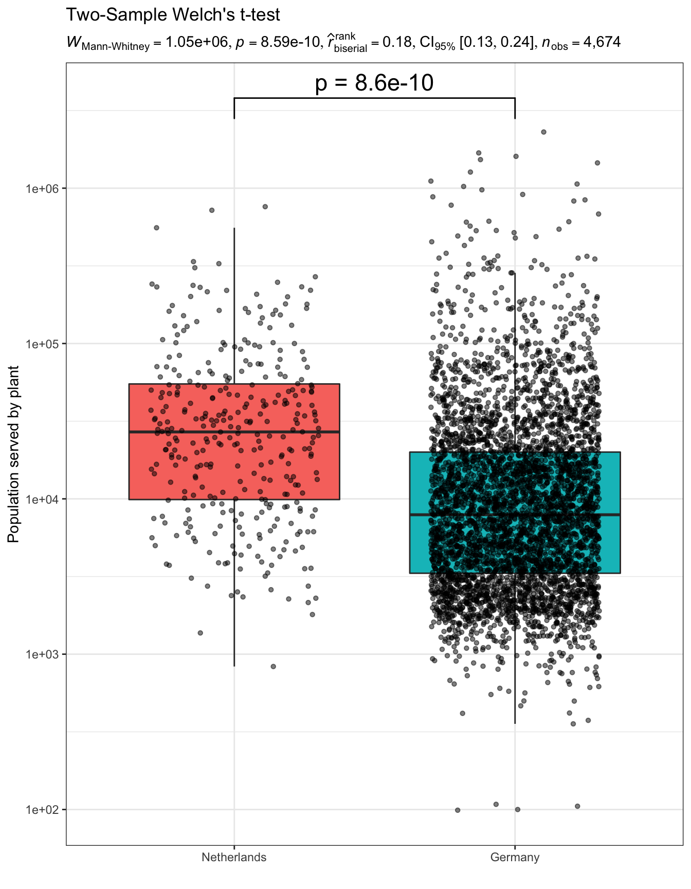
── Attaching packages ─────────────────────────────────────── tidyverse 1.3.2 ──
✔ ggplot2 3.3.6      ✔ purrr   0.3.4 
✔ tibble  3.1.8      ✔ dplyr   1.0.10
✔ tidyr   1.2.0      ✔ stringr 1.4.1 
✔ readr   2.1.2      ✔ forcats 0.5.1 
── Conflicts ────────────────────────────────────────── tidyverse_conflicts() ──
✖ dplyr::filter() masks stats::filter()
✖ dplyr::lag()    masks stats::lag()

Simple manipulation and visualization

colombian_wastes <- raw_data |> 
  mutate(COUNTRY = as_factor(COUNTRY), WASTE_ID = as_factor(WASTE_ID)) |> 
  filter(COUNTRY == "Colombia") |> 
  select(WASTE_ID, POP_SERVED, WASTE_DIS)

colombian_wastes |> 
  head() |> 
  knitr::kable()

WASTE_ID	POP_SERVED	WASTE_DIS
53476	1432	21.784
53679	3501	53.269
53680	25142	382.577
53681	42702	649.783
53682	89185	1357.091
53683	332964	5066.569

ggplot(colombian_wastes) +
  aes(y = reorder(WASTE_ID, POP_SERVED), x = POP_SERVED) +
  geom_col() +
  theme_minimal()

More advanced stuff

waste_pairs <- raw_data |> 
  mutate(COUNTRY = as_factor(COUNTRY), WASTE_ID = as_factor(WASTE_ID)) |> 
  filter(COUNTRY %in% c("Colombia", "Venezuela")) |> 
  select(COUNTRY, WASTE_ID, POP_SERVED, WASTE_DIS)

test_result <- statsExpressions::two_sample_test(
  waste_pairs, 
  COUNTRY, 
  POP_SERVED
  )

ggplot(waste_pairs) +
  aes(x = COUNTRY, y= POP_SERVED, fill = COUNTRY) +
  geom_boxplot(outlier.shape = NA) +
  geom_jitter(width = 0.3, alpha = 0.5, size = 1.2) +
  ggsignif::geom_signif(
    comparisons = list(c("Colombia", "Venezuela")),
    map_signif_level = TRUE, textsize = 6
  ) +
  labs(
    title = "Two-Sample Welch's t-test",
    subtitle = parse(text = test_result$expression),
    x = "",
    y = "Population served by plant"
  ) +
  theme_bw() +
  theme(
    legend.position = "none"
  )

Figure 1: Comparisons between Colombian and Venezuelan population benefited from waste water plants

Same as above

waste_pairs <- raw_data |> 
  mutate(COUNTRY = as_factor(COUNTRY), WASTE_ID = as_factor(WASTE_ID)) |> 
  filter(COUNTRY %in% c("Germany", "Netherlands")) |> 
  select(COUNTRY, WASTE_ID, POP_SERVED, WASTE_DIS)

test_result <- statsExpressions::two_sample_test(
  waste_pairs, 
  COUNTRY, 
  POP_SERVED, 
  type = "nonparametric"
  )

ggplot(waste_pairs) +
  aes(x = COUNTRY, y= POP_SERVED, fill = COUNTRY) +
  geom_boxplot(outlier.shape = NA) +
  geom_jitter(width = 0.3, alpha = 0.5, size = 1.2) +
  ggsignif::geom_signif(
    comparisons = list(c("Netherlands", "Germany")),
    # map_signif_level = TRUE, 
    map_signif_level = \(p) sprintf("p = %.2g", p),
    textsize = 6,
    test = "wilcox.test"
  ) +
  labs(
    title = "Two-Sample Welch's t-test",
    subtitle = parse(text = test_result$expression),
    x = "",
    y = "Population served by plant"
  ) +
  theme_bw() +
  theme(
    legend.position = "none"
  ) +
  scale_y_log10()

Figure 2: Comparisons between German and Dutch population benefited from waste water plants

Some conclusions

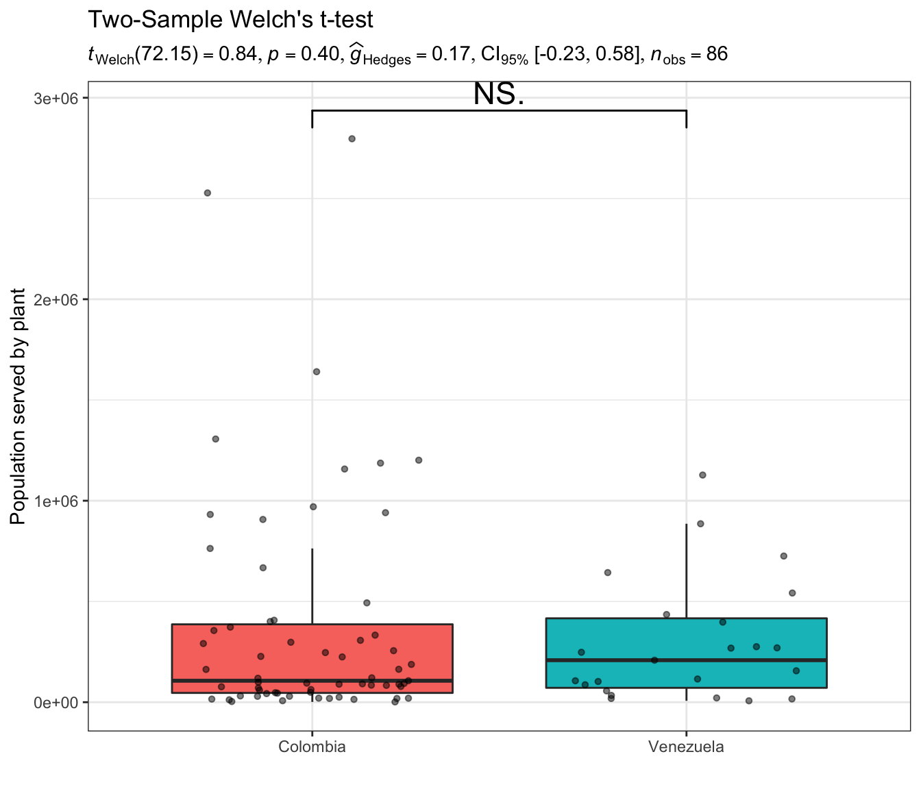
From the comparison between Colombia vs Venezuela benefited population from waste water plants Fig. 1, there are at least two important highlights. First, both countries display relatively low numbers plants given their extensions (this is something more of an intuition coming from the other comparisons as well), and a second thing is that there is actually no differences regarding the population they are attending. The opposite happens when comparing Germany vs. Netherlands benefited populations Fig. 2.

Citation

BibTeX citation:

@misc{garcía-botero2021,
  author = {García-Botero, Camilo},
  title = {Population Benefited from Waste Water Plants},
  date = {2021-09-20},
  url = {https://camilogarciabotero.github.io/blog},
  langid = {en}
}

For attribution, please cite this work as:

García-Botero, Camilo. 2021. “Population Benefited from Waste Water Plants.” https://camilogarciabotero.github.io/blog.