Artists in the USA

Camilo García-Botero

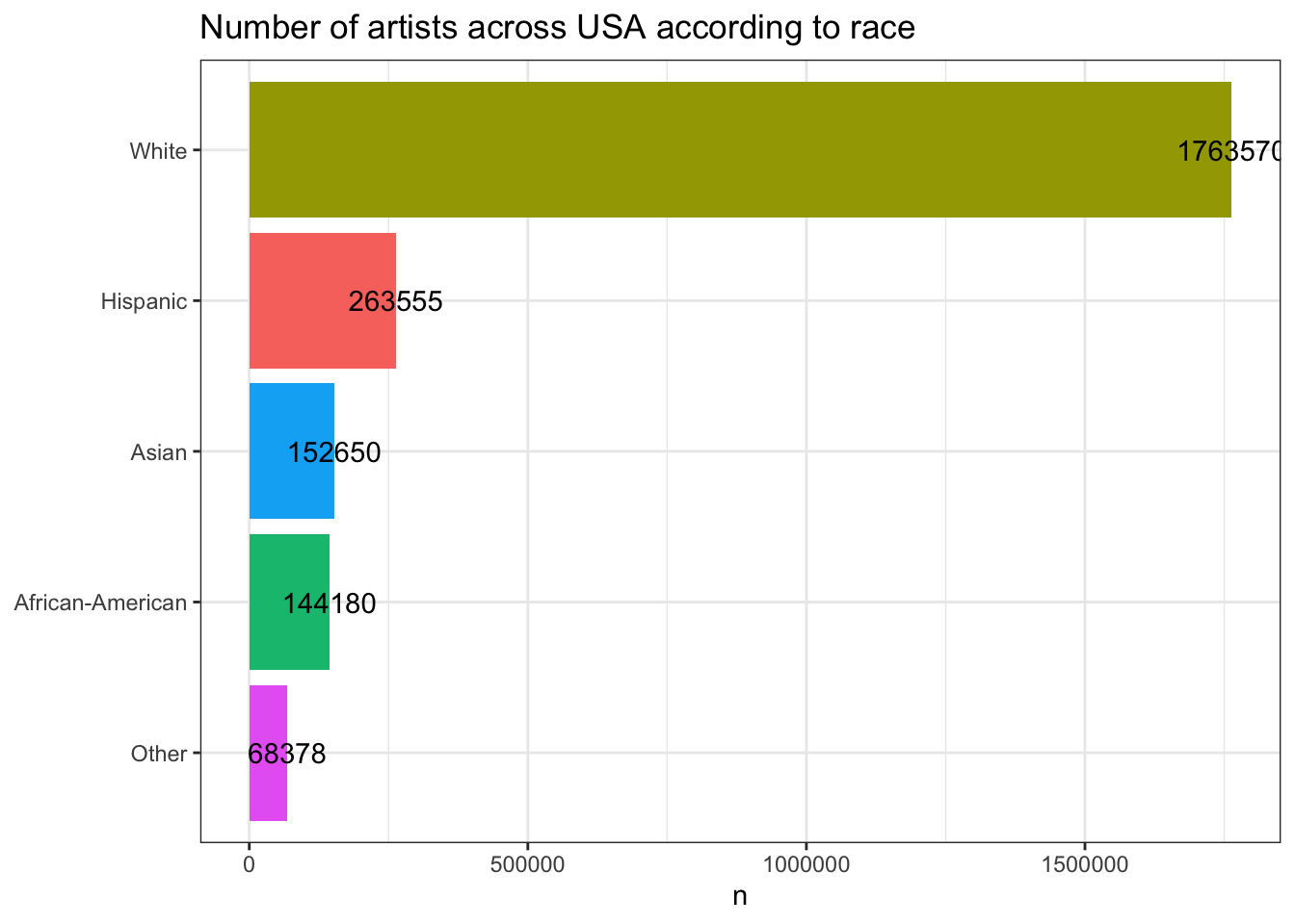
This post covers the code and figures from the datascience workshop with R, where we explore some basics from dplyr and ggplot2 packages using the tidytuesday data set from the current week (2021-09-27).

Importing libraries

library(tidyverse)

── Attaching packages ─────────────────────────────────────── tidyverse 1.3.2 ──
✔ ggplot2 3.3.6      ✔ purrr   0.3.4 
✔ tibble  3.1.8      ✔ dplyr   1.0.10
✔ tidyr   1.2.0      ✔ stringr 1.4.1 
✔ readr   2.1.2      ✔ forcats 0.5.1 
── Conflicts ────────────────────────────────────────── tidyverse_conflicts() ──
✖ dplyr::filter() masks stats::filter()
✖ dplyr::lag()    masks stats::lag()

Importing data from TT

artists <- readr::read_csv("https://raw.githubusercontent.com/rfordatascience/tidytuesday/master/data/2022/2022-09-27/artists.csv")

Rows: 3380 Columns: 7
── Column specification ────────────────────────────────────────────────────────
Delimiter: ","
chr (3): state, race, type
dbl (4): all_workers_n, artists_n, artists_share, location_quotient

ℹ Use `spec()` to retrieve the full column specification for this data.
ℹ Specify the column types or set `show_col_types = FALSE` to quiet this message.

artists

Data manipulation

all_artists <- artists |>
  mutate(across(state:type, as_factor)) |>
  drop_na(artists_n) |>
  group_by(race) |>
  summarize(n = sum(artists_n))

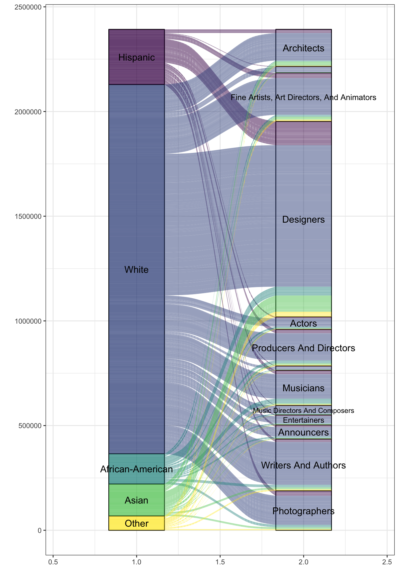
all_artists

Data visualization

ggplot(all_artists) +
  aes(y = reorder(race, n), x = n, fill = race, label = n) +
  geom_col() +
  geom_text() +
  theme_bw() +
  theme(
    legend.position = "none",
    axis.title.y = element_blank()
  ) +
  labs(
    title = "Number of artists across USA according to race"
  )

Alluvial plots

factored_artists <- artists |>
  mutate(across(state:type, as_factor)) |> 
  group_by(race, type, state) |> 
  summarise(artists_n) |>
  drop_na()

`summarise()` has grouped output by 'race', 'type'. You can override using the
`.groups` argument.

library(ggalluvial)
library(ggfittext)

ggplot(factored_artists) +
  aes(y = artists_n, axis1 = race, axis2 = type, fill = race) +
  geom_stratum(alpha = .5) +
  geom_alluvium() +
  geom_fit_text(stat = "stratum", aes(label = after_stat(stratum))) +
  theme_bw() +
  theme(
    legend.position = "none"
  ) +
  scale_fill_viridis_d() +
  labs(
    y = ""
  )

Citation

BibTeX citation:

@misc{garcía-botero2021,
  author = {García-Botero, Camilo},
  title = {Artists in the {USA}},
  date = {2021-09-27},
  url = {https://camilogarciabotero.github.io/blog},
  langid = {en}
}

For attribution, please cite this work as:

García-Botero, Camilo. 2021. “Artists in the USA.” https://camilogarciabotero.github.io/blog.