An introduction to R

https://bit.ly/3ZRsbnA

Camilo G.

ca.garcia2@uniandes.edu.co

Kevin J.

ks.jaramillo1905@uniandes.edu.co

Victor A.

v.nascimento@uniandes.edu.co

R and Rstudio

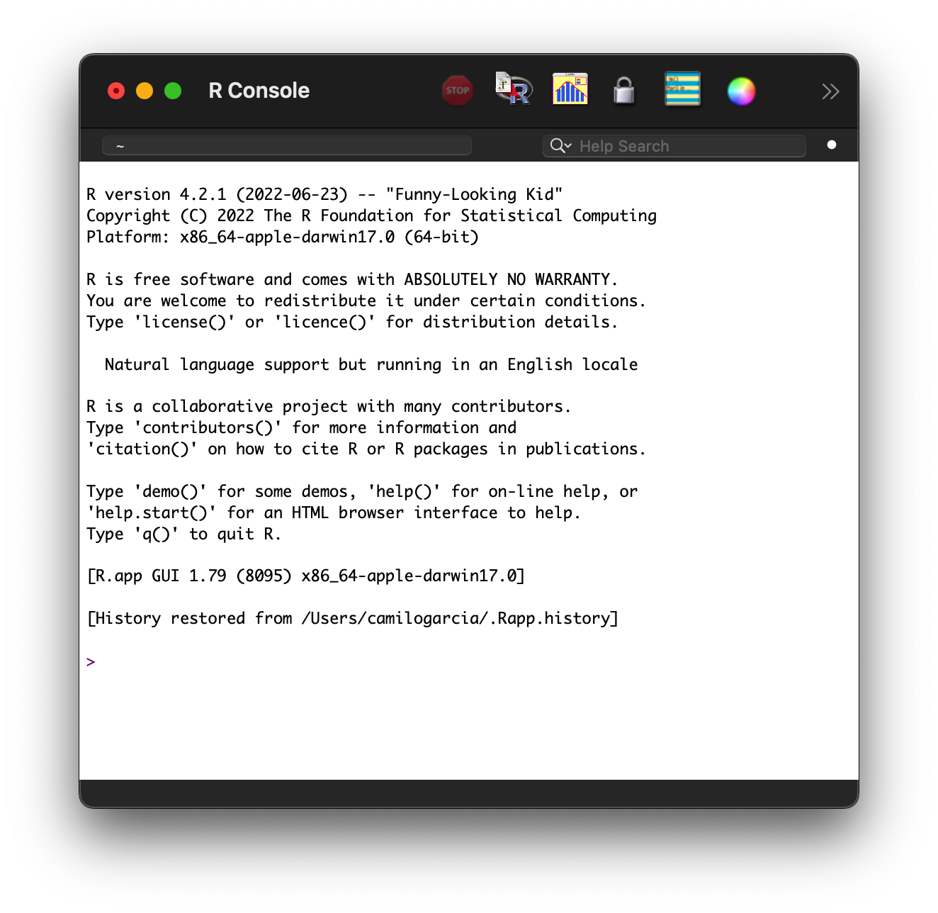
R console

Rstudio IDE

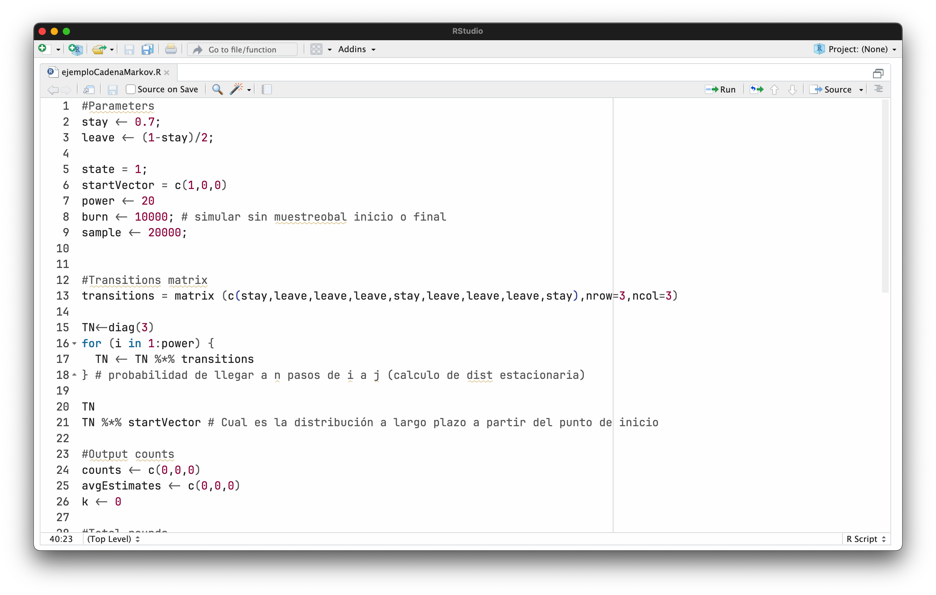
An script example

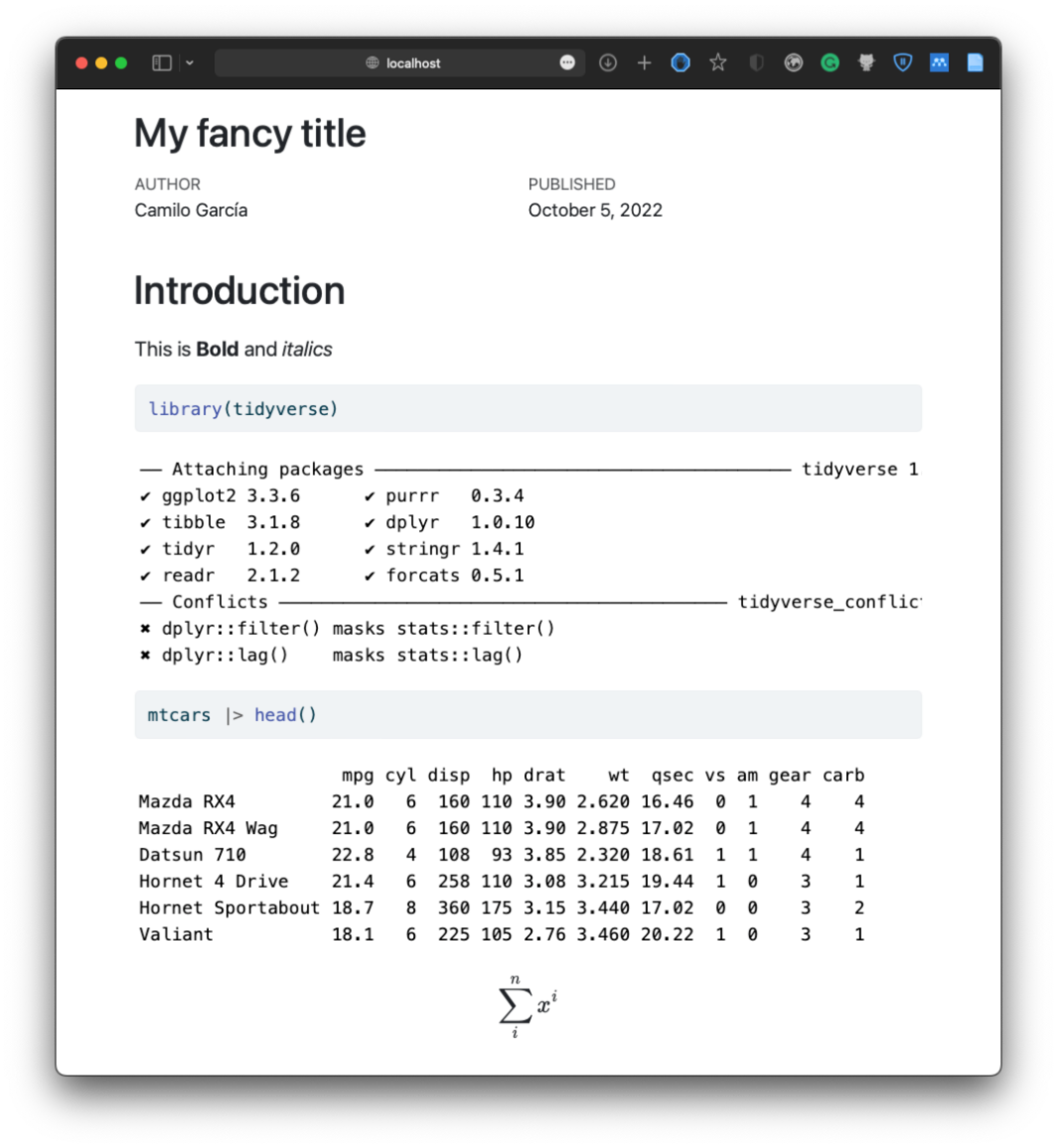
Rmarkdown and Dynamic Documents

The YAML block

---
title: ”My fancy title"
author: "Camilo García"
format: html
date: 2022-10-05
---

Simple text (in Markdown)

# Introduction

This is **Bold** and *italics*

Code

library(tidyverse)
mtcars |> head()

LaTeX

$$
\sum_{i}^{n} x^{i}
$$

Installing Packages

Two main commands are used to manage packages in R:

Installation:

install.packages("pkgname")

Loading the package:

library(pkgname)

Getting Help

help(function)
?function
help.search(“keyword”)

Important Syntax

Creating Objects

Anything that is created in R whether it is a vector, matrix, function, data, figures, strings (character), etc. can be assigned into an object using the <- operator:

name <- "camilo"
name

[1] "camilo"

typeof(name)

[1] "character"

Main Objects in R

Vectors

A vector is a concatenation of other objects of the same type.

time <- c(34, 13, 65, 10)

season <- c("dry", "semidry", "rainy")

heights  <- c(1.60, 1.63, 1.85 ,1.72)

Matrices

A matrix is an array of objects that are ordered in rows and columns

mx <- matrix(
    c(23, 58, 98, 54, 68, 74),
    nrow = 2,
    ncol = 3,
    byrow = FALSE,
    dimnames = list(
        rows = c("rw1", "rw2"),
        cols = c("cl1", "cl2", "cl3")
    )
)

mx

     cols
rows  cl1 cl2 cl3
  rw1  23  98  68
  rw2  58  54  74

Lists

A list is a set of ordered components (objects with assignments)

student_info  <- list(name = "Alejandro", exam = 5, quizzes = c(4,5,3.5,4.2))
student_info

$name
[1] "Alejandro"

$exam
[1] 5

$quizzes
[1] 4.0 5.0 3.5 4.2

Managing Data

Manually Generated Data

The seq() function can be used to create a sequence of data:

data  <- seq(1,100,10) 
data

 [1]  1 11 21 31 41 51 61 71 81 91

The rep() function creates repetitions of an object $n$ times

data  <- rep("Ho", 3)
data

[1] "Ho" "Ho" "Ho"

You can also generate factors/levels using the gl() function.

gl(
    n, # levels 
    k, # replications
    length = n * k,
    labels = c("contro", "treatment"),
    ordered = FALSE
)

let’s try an example:

## First control, then treatment:
#| output-location: fragment
experiment <- gl(2, 8, labels = c("Control", "Treat"))

experiment

 [1] Control Control Control Control Control Control Control Control Treat  
[10] Treat   Treat   Treat   Treat   Treat   Treat   Treat  
Levels: Control Treat

The data.frame object is a native structure/object to store table like data

size  <- c(34,50,40)
color  <- c("blue", "red", "orange")

frogs  <- data.frame(size, color)

frogs

Importing Data

There are many function to import data to the R session. read.table() is one of the basic ones:

spp_data <- read.table(
  file = "data/especies.txt",
  sep = "\t",
  h = TRUE
)
spp_data

We can select subsets of the data set using many strategies.

The $ operator for column subseting:

spp_data$Especie

 [1] "C_fitzingeri"  "D_ebraccatus"  "E_pustulosus"  "O_histrionica"
 [5] "S_phaeota"     "C_fitzingeri"  "D_ebraccatus"  "E_pustulosus" 
 [9] "O_histrionica" "S_phaeota"     "C_fitzingeri"  "D_ebraccatus" 
[13] "E_pustulosus"  "O_histrionica" "S_phaeota"     "C_fitzingeri" 
[17] "D_ebraccatus"  "E_pustulosus"  "O_histrionica" "S_phaeota"    
[21] "C_fitzingeri"  "D_ebraccatus"  "E_pustulosus"  "O_histrionica"
[25] "S_phaeota"

The indexed way:

spp_data[,2]

 [1] "C_fitzingeri"  "D_ebraccatus"  "E_pustulosus"  "O_histrionica"
 [5] "S_phaeota"     "C_fitzingeri"  "D_ebraccatus"  "E_pustulosus" 
 [9] "O_histrionica" "S_phaeota"     "C_fitzingeri"  "D_ebraccatus" 
[13] "E_pustulosus"  "O_histrionica" "S_phaeota"     "C_fitzingeri" 
[17] "D_ebraccatus"  "E_pustulosus"  "O_histrionica" "S_phaeota"    
[21] "C_fitzingeri"  "D_ebraccatus"  "E_pustulosus"  "O_histrionica"
[25] "S_phaeota"

Using a subset() and a condition:

subset(spp_data, Prob_presencia > 0)

Common Operations

85+12

[1] 97

56-29

[1] 27

8*8

[1] 64

70/100

[1] 0.7

2^4

[1] 16

Importance of precedence

2+3*2-2^3

[1] 0

((2+3)*2-2)^3

[1] 512

Operations with vectors:

time <- c(34, 13, 65, 10)
time + 5

[1] 39 18 70 15

What if you want to add another value to the vector:

time[5] = 5
time

[1] 34 13 65 10  5

So, the vector is now bigger:

length(time)

[1] 5

Descriptive Stats

The simplest way to generate descriptive stats of a dataset is using summary() function.

summary(spp_data)

      Zona     Especie          Prob_presencia      variacion    
 Min.   :1   Length:25          Min.   :0.01996   Min.   :11.00  
 1st Qu.:2   Class :character   1st Qu.:0.27549   1st Qu.:33.00  
 Median :3   Mode  :character   Median :0.42008   Median :59.00  
 Mean   :3                      Mean   :0.46289   Mean   :52.57  
 3rd Qu.:4                      3rd Qu.:0.65240   3rd Qu.:72.50  
 Max.   :5                      Max.   :0.92721   Max.   :89.00  
                                NA's   :1         NA's   :2

Inspecting Data

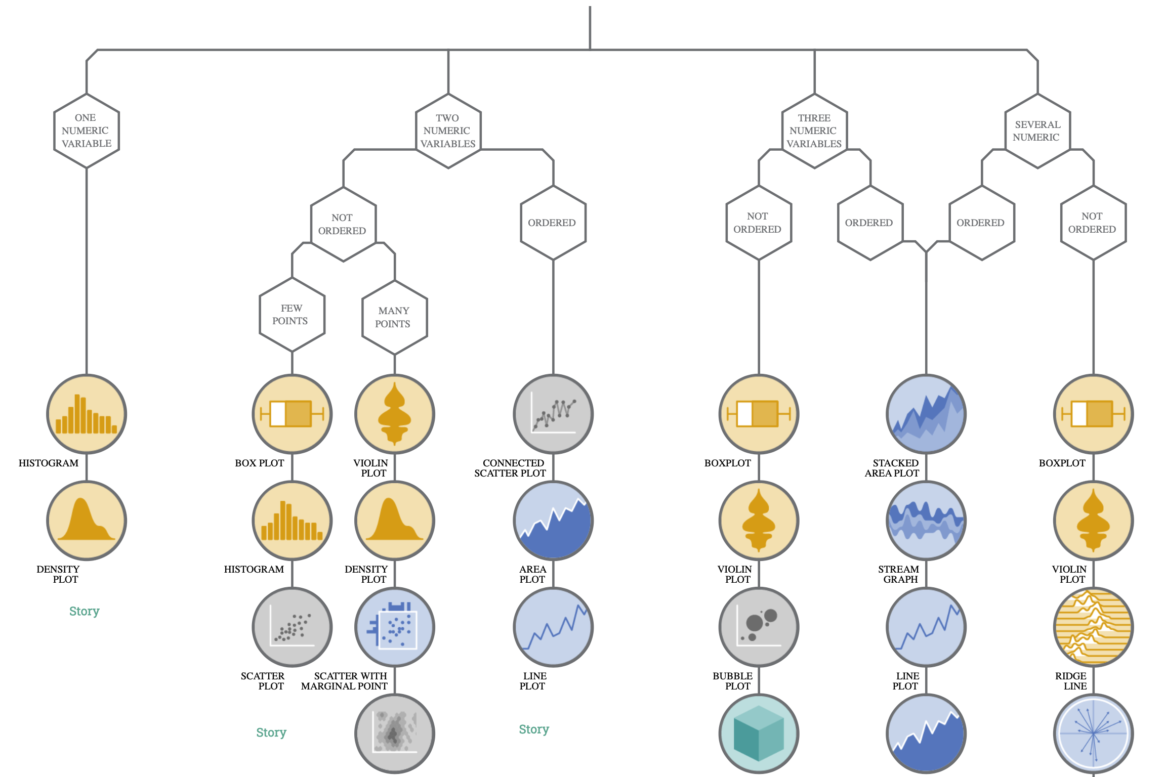
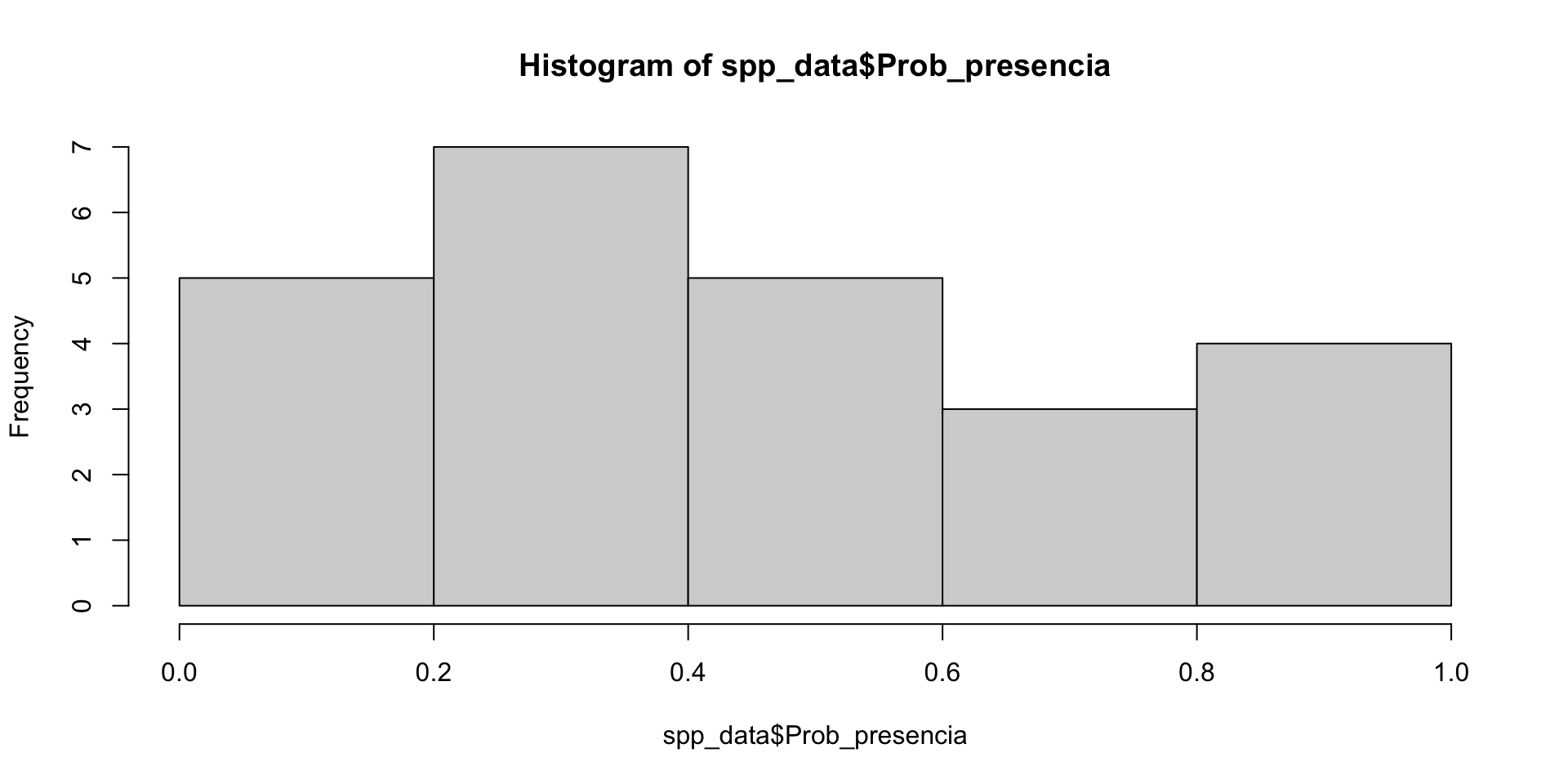
Let’s create an histogram, using base hist() function: