Descriptive Stats & Distributions

http://tinyurl.com/4dfuycvt

Camilo G.

ca.garcia2@uniandes.edu.co

Ada A.

a.acevedoa2@uniandes.edu.co

Ronald D.

r.diazf@uniandes.edu.co

Descriptive stats

Mean & Median

Sample mean: \[ \overline{x} = \frac{1}{n}\sum^{n}_{i=1}x_{i} \]

You can create the function:

new_mean <- function(x){sum(x)/length(x)}

new_mean(penguins$year)

[1] 2008.029

Or simply use a predefined mean:

mean(penguins$year, na.rm=TRUE)

[1] 2008.029

Sample median: \[ median= \begin{cases} x_{(n+1)/2} &\text{if $n \equiv 1$} \\ \frac{(x_{n/2} + x_{((n/2)+1)})}{2} &\text{if $n \equiv 0$} \end{cases} \]

In R a freshly defined function:

new_median <- function(x) {
  if(length(x) %% 2 != 0){
   (sort(x)[length(x)/2] + sort(x)[(length(x)/2)+1])/2
      } else{
       sort(x)[ceiling(length(x)/2)]
    }
   }

1

The operator %% is called modulus. In this case, will return the remainder of the division (in this case by 2), and then will check if this value is different than 0. If so, then will apply the equation for the odd-numbered list.

2

Equation for n if it is odd

3

Equation for n if it is even

new_median(penguins$body_mass_g)

[1] 4050

Or the predefined function

median(penguins$body_mass_g, na.rm = TRUE)

[1] 4050

Variance, Standard deviation & Variation coefficient

Sample variance (unbiased): \[ S^{2} = \frac{1}{n-1}\sum^{n}_{i=1}(x_{i}-\overline{x})^{2} \]

var(penguins$body_mass_g, na.rm=TRUE)

[1] 643131.1

Standard deviation

\[ S = \sqrt{\frac{1}{n-1}\sum^{n}_{i=1}(x_{i}-\overline{x})^{2}} \]

sd(penguins$body_mass_g, na.rm=TRUE)

[1] 801.9545

Variation coefficient

\[ CV = \frac{S}{\overline{x}} \times 100 \]

cv <- function(x, na.rm=TRUE){(sd(x, na.rm=TRUE)/mean(x, na.rm=TRUE))*100}

cv(penguins$body_mass_g, na.rm=TRUE)

[1] 19.08618

Confidence intervals

Estimates the range within which a population parameter is likely to fall. It provides a way to express the uncertainty or margin of error associated with a sample estimate. \[ \text{IC} = \bar{x} \pm Z \left( \frac{\sigma}{\sqrt{n}} \right) \]

Or if the population standard deviation of the population is unknown:

\[ \text{IC} = \bar{x} \pm t \left( \frac{s}{\sqrt{n}} \right) \]

Using dplyr for summarizing stats

library(dplyr)

penguins |>
    group_by(species)

penguins |>
    group_by(species) |>
    summarise(
        mean_body_mass_g = mean(body_mass_g, na.rm = TRUE)
        )

penguins |>
    group_by(species) |>
    summarise(
        mean_body_mass_g = mean(body_mass_g, na.rm = TRUE),
        variance_body_mass_g = var(body_mass_g, na.rm = TRUE)
        )

penguins |>
    group_by(species) |>
    summarise(
        mean_body_mass_g = mean(body_mass_g, na.rm = TRUE),
        variance_body_mass_g = var(body_mass_g, na.rm = TRUE),
        std_dev_body_mass_g = sd(body_mass_g, na.rm = TRUE)
        )

penguins |>
    group_by(species) |>
    summarise(
        mean_body_mass_g = mean(body_mass_g, na.rm = TRUE),
        variance_body_mass_g = var(body_mass_g, na.rm = TRUE),
        std_dev_body_mass_g = sd(body_mass_g, na.rm = TRUE),
        cv_body_mass_g = cv(body_mass_g, na.rm = TRUE)
        )

Distributions

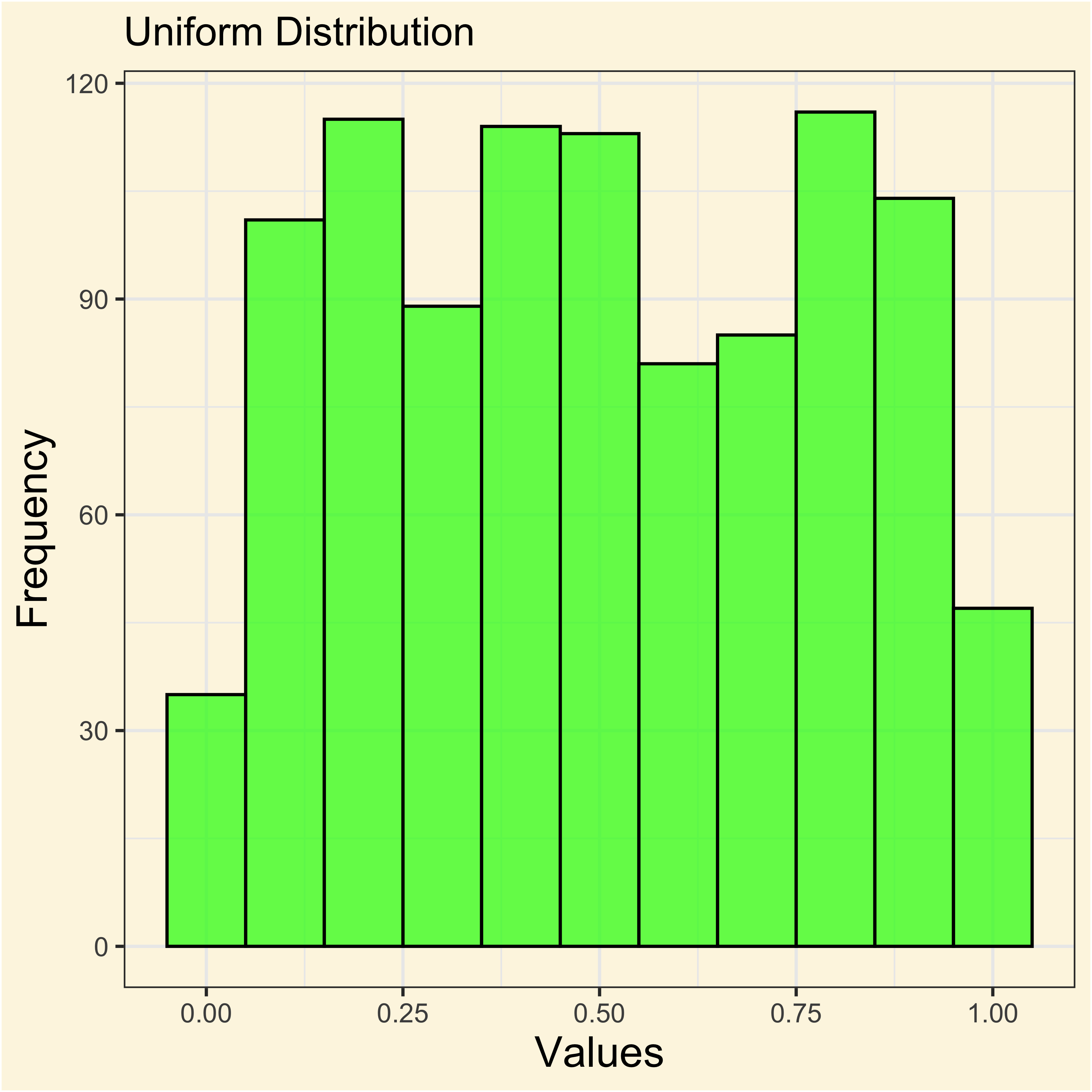
dfuniform <- runif(1000, min = 0, max = 1)

ggplot(data.frame(x = dfuniform), aes(x)) +
  geom_histogram(
    binwidth = 0.1, 
    fill = "green", 
    color = "black", 
    alpha = 0.7
  ) +
  labs(
    title = "Uniform Distribution",
    x = "Values",
    y = "Frequency"
  )

dfbin <- rbinom(1000, size = 20, prob = 0.8)

ggplot(data.frame(x = dfbin), aes(x)) +
  geom_histogram(
    binwidth = 1, 
    fill = "purple", 
    color = "black", 
    alpha = 0.7
  ) +
  labs(
    title = "Binomial Distribution",
    x = "Values",
    y = "Frequency"
  )

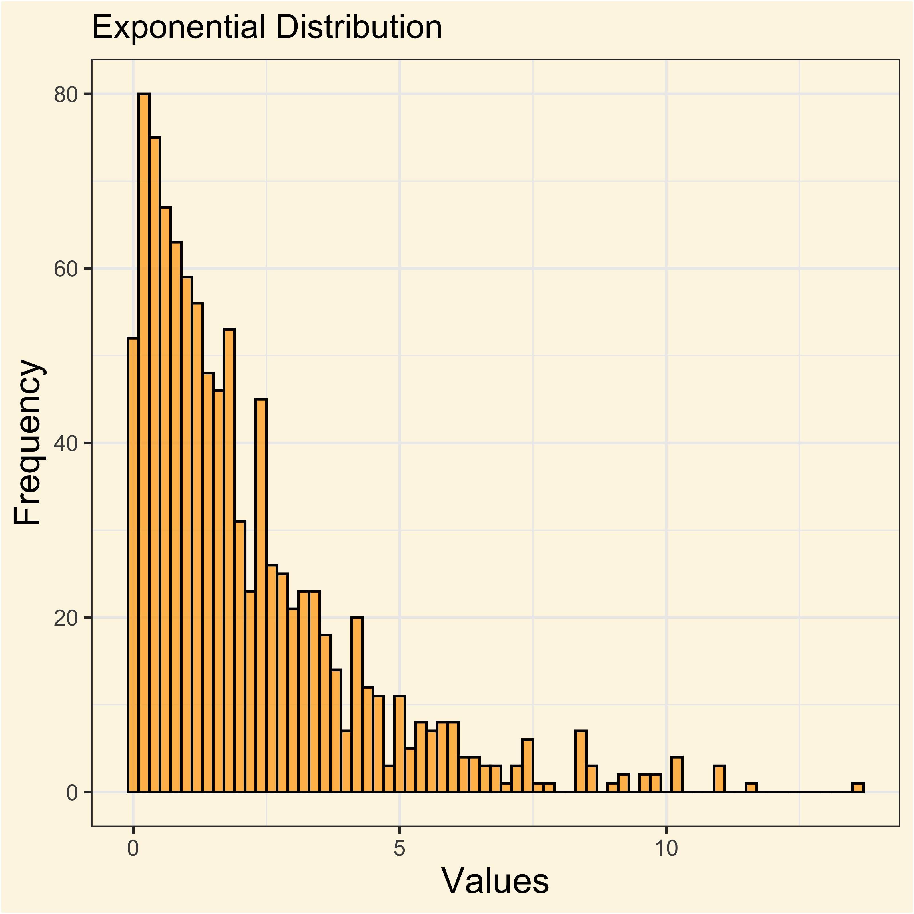
dfexp <- rexp(1000, rate = 0.5)

ggplot(data.frame(x = dfexp), aes(x)) +
  geom_histogram(
    binwidth = 0.2,
    fill = "orange", 
    color = "black", 
    alpha = 0.7
  ) +
  labs(
    title = "Exponential Distribution",
    x = "Values",
    y = "Frequency"
  )

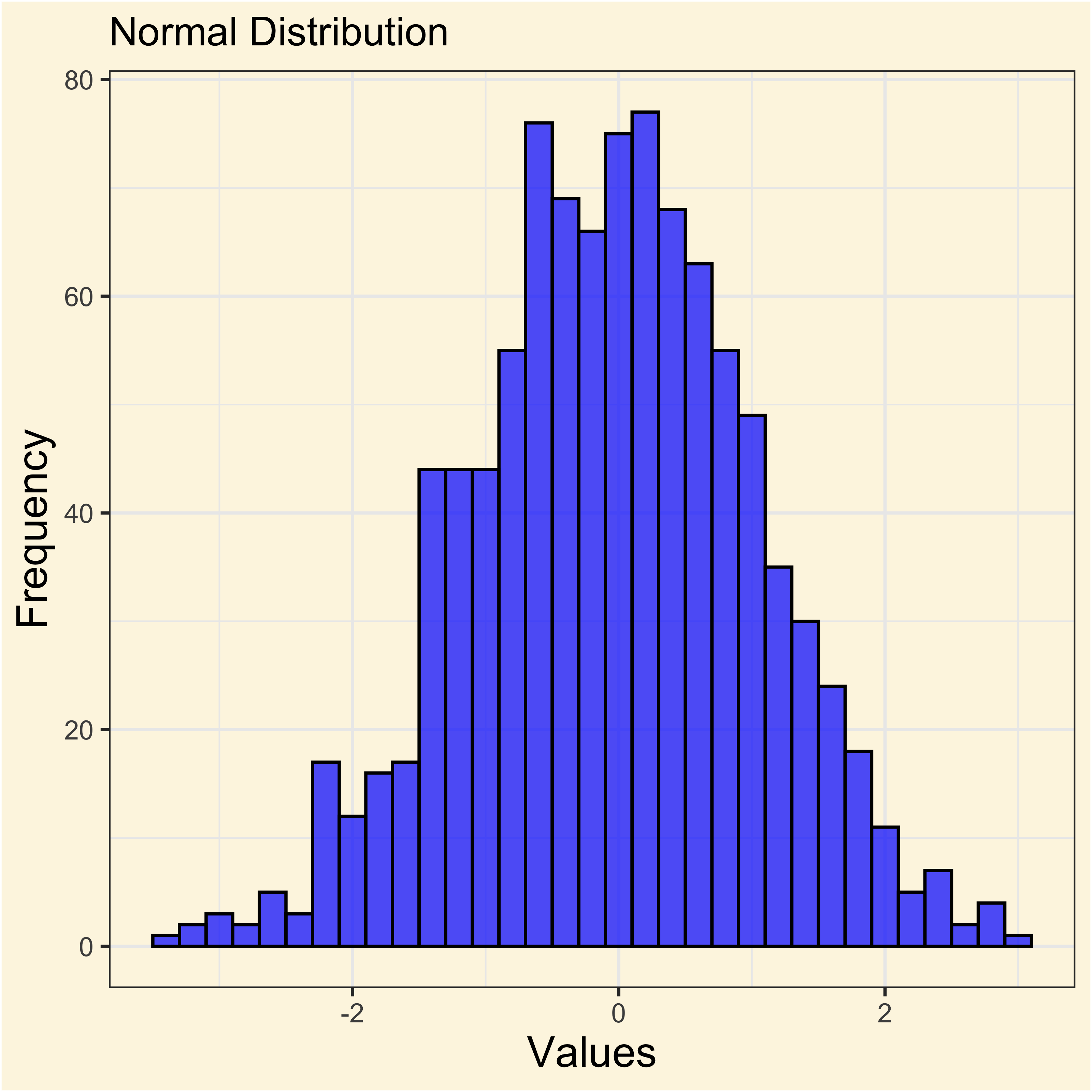
dfnormal <- rnorm(1000, mean = 0, sd = 1)

ggplot(data.frame(x = dfnormal), aes(x)) +
  geom_histogram(
    binwidth = 0.2, 
    fill = "blue", 
    color = "black", 
    alpha = 0.7
  ) +
  labs(
    title = "Normal Distribution",
    x = "Values",
    y = "Frequency"
  )

The standard normal distribution

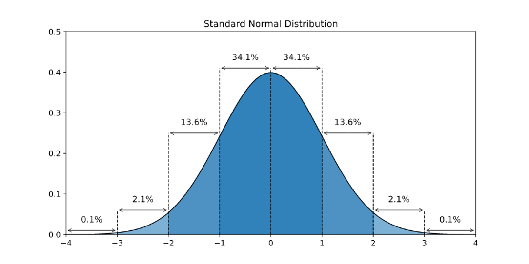
Where \(z = \frac{x - \mu} {\sigma}\) is the standardization function, the result is that \(\sigma = 1\) and \(\mu = 0\)

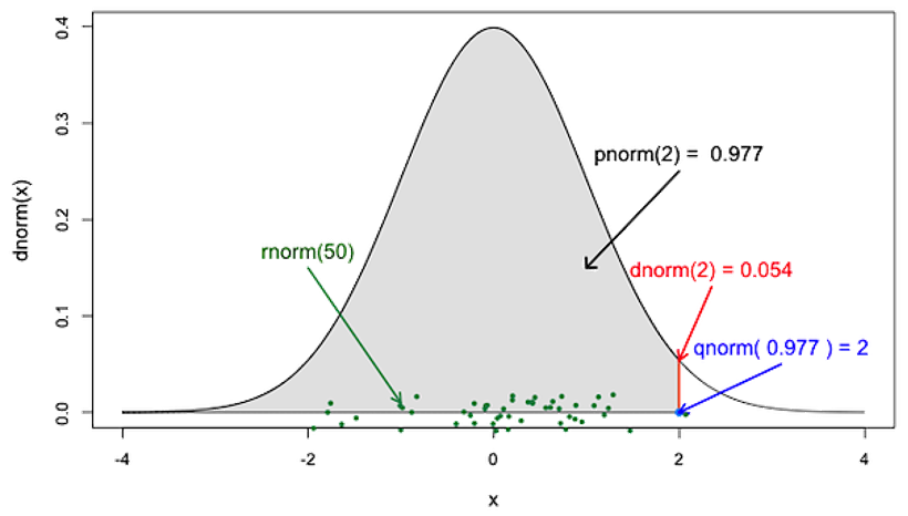
family of normality functions in R

• rnorm() generates pseudorandom normal numbers.
• dnorm() is the probability density function (PDF)
• pnorm() is the cumulative density function
• qnorm() calculates the quantile of the normal distribution

Let’s try with an example:

Now, the Adelie penguins display an average bill length of 38.8 mm and its standard variation is 2.6 mm. What’s the percentage of penguins of 40 mm or smaller?

pnorm(40, mean = 38.8, sd = 2.6)

[1] 0.6777938

When the frequencies of a random variable \(X\) cluster around a central value, it is said that it follows a normal distribution.

In summary a variable that appears to follow a normal distribution displays three properties:

1. Most values clustered around the average.
2. Extreme values are less frequent, but not impossibles.
3. Distribution display are quite symmetric from the mean.