Correlation & Lineal regression

https://bit.ly/3IlpxQ5

Camilo G.

ca.garcia2@uniandes.edu.co

Ada A.

a.acevedoa2@uniandes.edu.co

Ronald D.

r.diazf@uniandes.edu.co

Correlation

Correlation is a measurement of the extent of which two variables relate to each other. Its coefficient tells the direction and strength of this relationship.

ggplot(penguins, aes(x = bill_length_mm, y = bill_depth_mm)) +
    geom_point(size = 2, alpha = 0.6) +
    labs(
        title = "Penguin bill dimensions (omit species)",
        x = "Bill length (mm)",
        y = "Bill depth (mm)"
    ) +
    geom_smooth(method = "lm", se = FALSE, color = "gray50")

How much are those variables correlated?

The Pearson correlation coefficient

The Pearson correlation coefficient stablish the degree of correlation between two random variables:

\[ \rho_{X,Y} = \frac{Cov(X,Y)}{\sigma_{X}\sigma_{Y}} \]

In R:

cor.test(penguins$bill_length_mm, penguins$bill_depth_mm, method = "pearson")

    Pearson's product-moment correlation

data:  penguins$bill_length_mm and penguins$bill_depth_mm
t = -4.4591, df = 340, p-value = 1.12e-05
alternative hypothesis: true correlation is not equal to 0
95 percent confidence interval:
 -0.3328072 -0.1323004
sample estimates:
       cor 
-0.2350529 

The Pearson Correlation assumptions:

• \(X\) and \(Y\) display a linear tendency.
• \(X\) and \(Y\) display a normal distribution.

The Spearman correlation coefficient

\[ \rho_{X,Y} = \frac{Cov(R(X),R(Y))}{\sigma_{R(X)}\sigma_{R(Y)}} \]

The \(R\) in the equation is a ranking of the the two random variables.

In R:

cor.test(penguins$bill_length_mm, penguins$bill_depth_mm, method = "spearman")

    Spearman's rank correlation rho

data:  penguins$bill_length_mm and penguins$bill_depth_mm
S = 8145268, p-value = 3.512e-05
alternative hypothesis: true rho is not equal to 0
sample estimates:
       rho 
-0.2217492 

Linear regression

Before dive into the linear regression model creation and the hypothesis testing. Let’s talk about two important principles for sampling in the experimental design you are performing.

1. Capture full ranges of response

2. Sample range uniformly

Linear regression model

The linear regression model is a statistical model that allows us to predict the value of a dependent variable \(Y\) based on the value of an independent variable \(X\).

Applying the linear regression model

Finding the best fit

Testing the hypothesis in linear regression

How do we test if the SSreg (\(𝐻_{𝐴}\)) explain the data trend?

or, in other words…

How do we test if the \(𝐻_{0}\) do not explain the data trend?

1. Specifying the statistical test

\[ F_{(df,n)} = \frac{SS_{reg}}{\frac{RSS}{(n − 2)}} \]

2. Calculating the tail probability in T-distribution

\[ X \sim F_{(1,n)} \Rightarrow X \sim T_{n} \]

Let’s do it in R

ggplot(penguins, 
  aes(
      x = flipper_length_mm, 
      y = body_mass_g)
      ) +
    geom_point(size = 2, alpha = 0.6) +
    labs(
        title = "Penguin bill dimensions",
        x = "flipper length (mm)",
        y = "Body mass (g)"
    ) +
    geom_smooth(method = "lm")

Let’s investigate the model:

model  <- lm(body_mass_g ~ flipper_length_mm, data = penguins)

Call:
lm(formula = body_mass_g ~ flipper_length_mm, data = penguins)

Coefficients:
      (Intercept)  flipper_length_mm  
         -5780.83              49.69  

We can use the package report to get a nice summary of the model:

report::report(model)

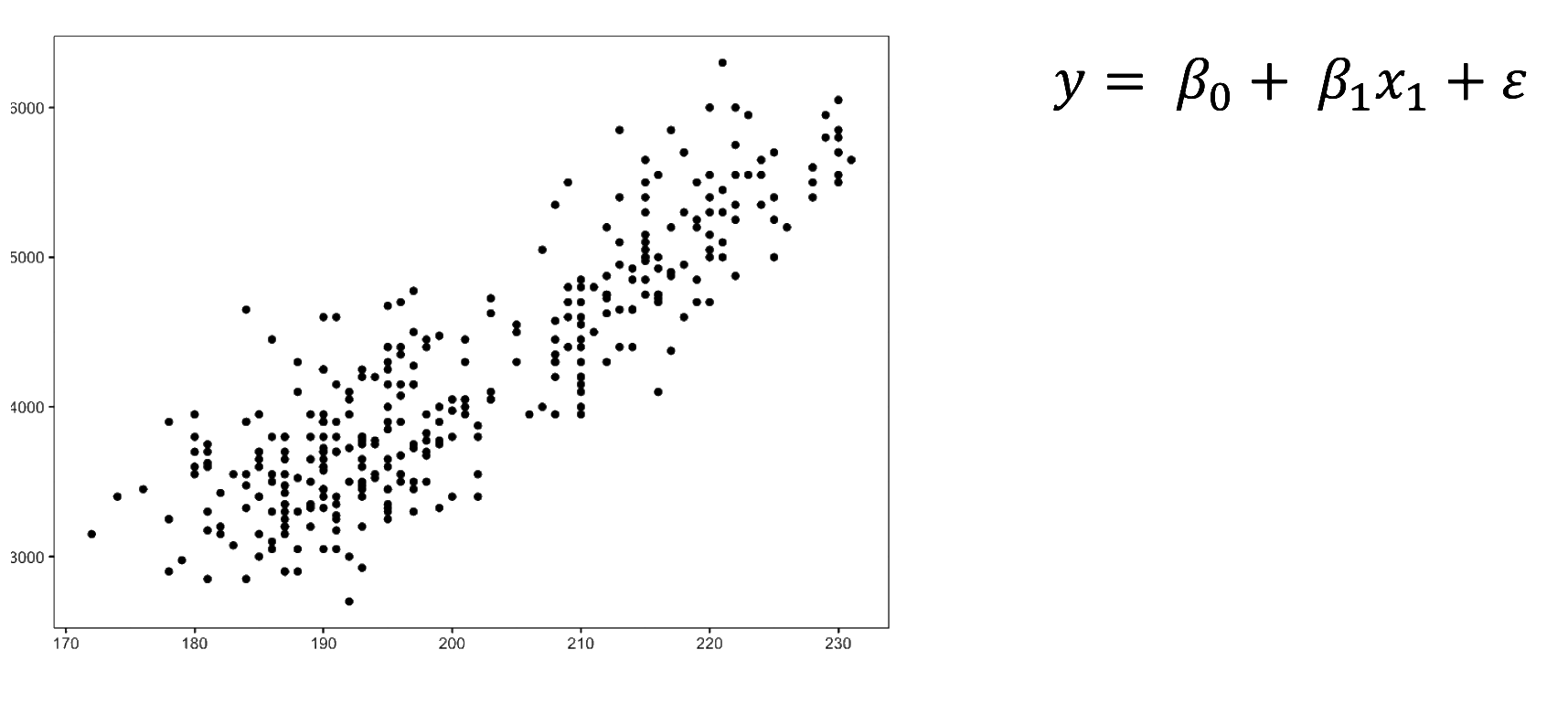
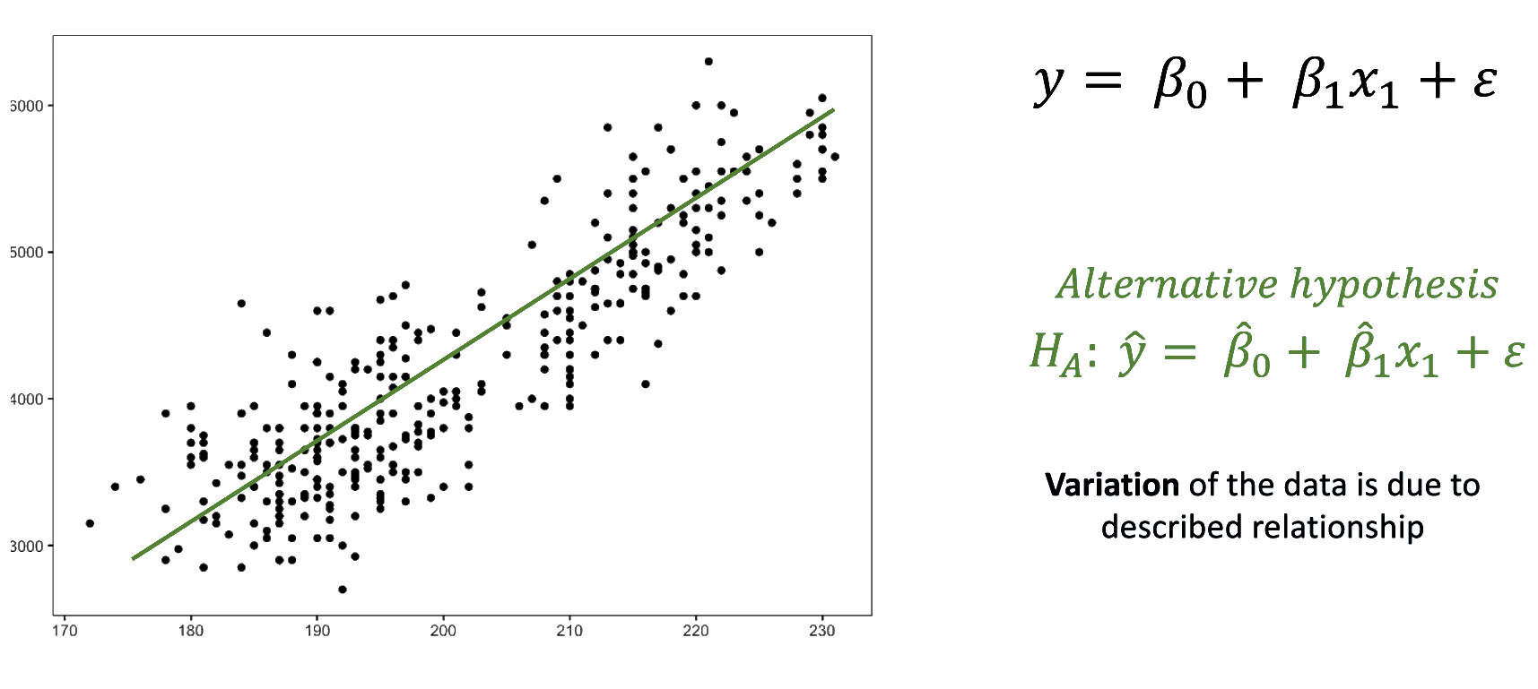
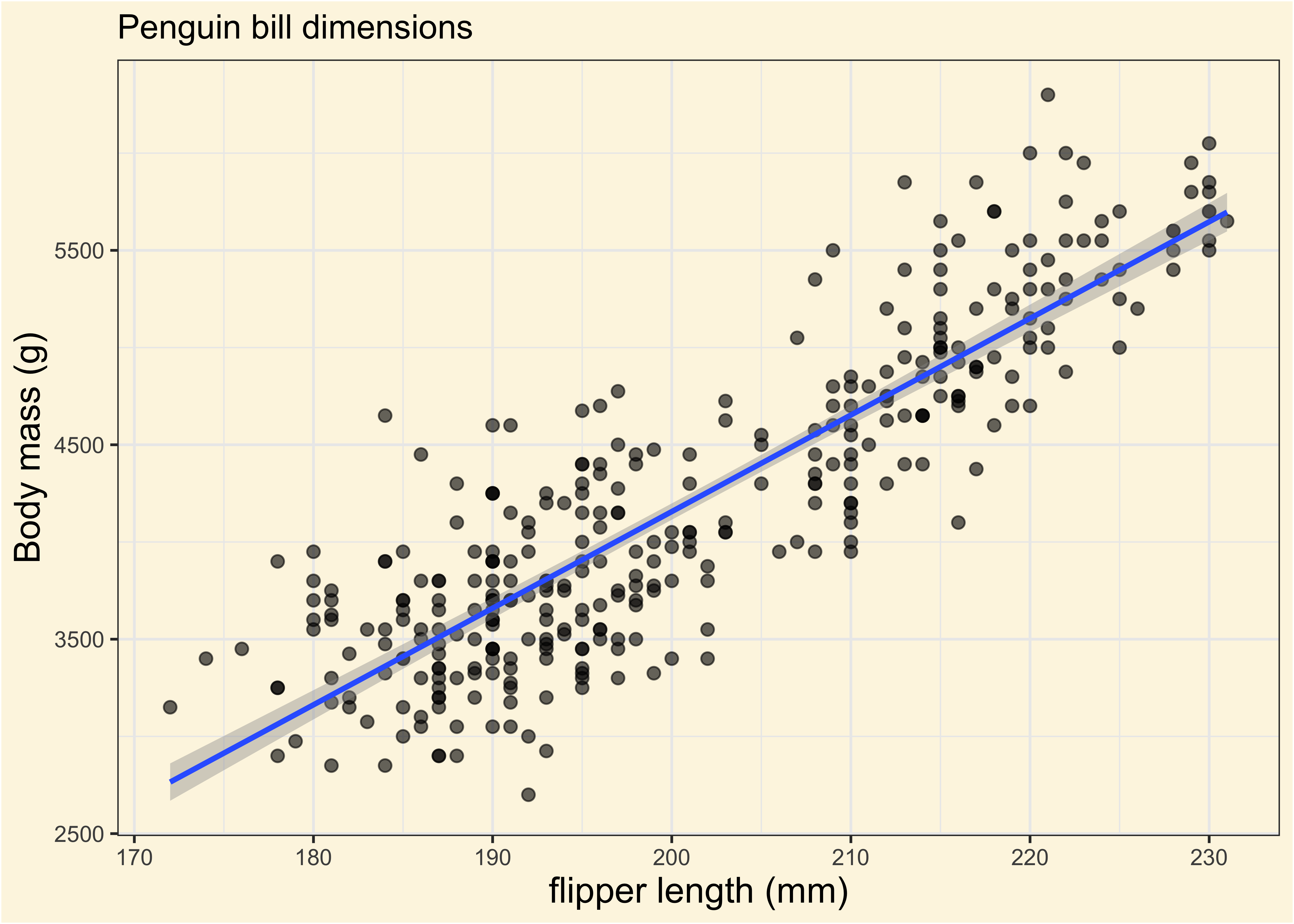
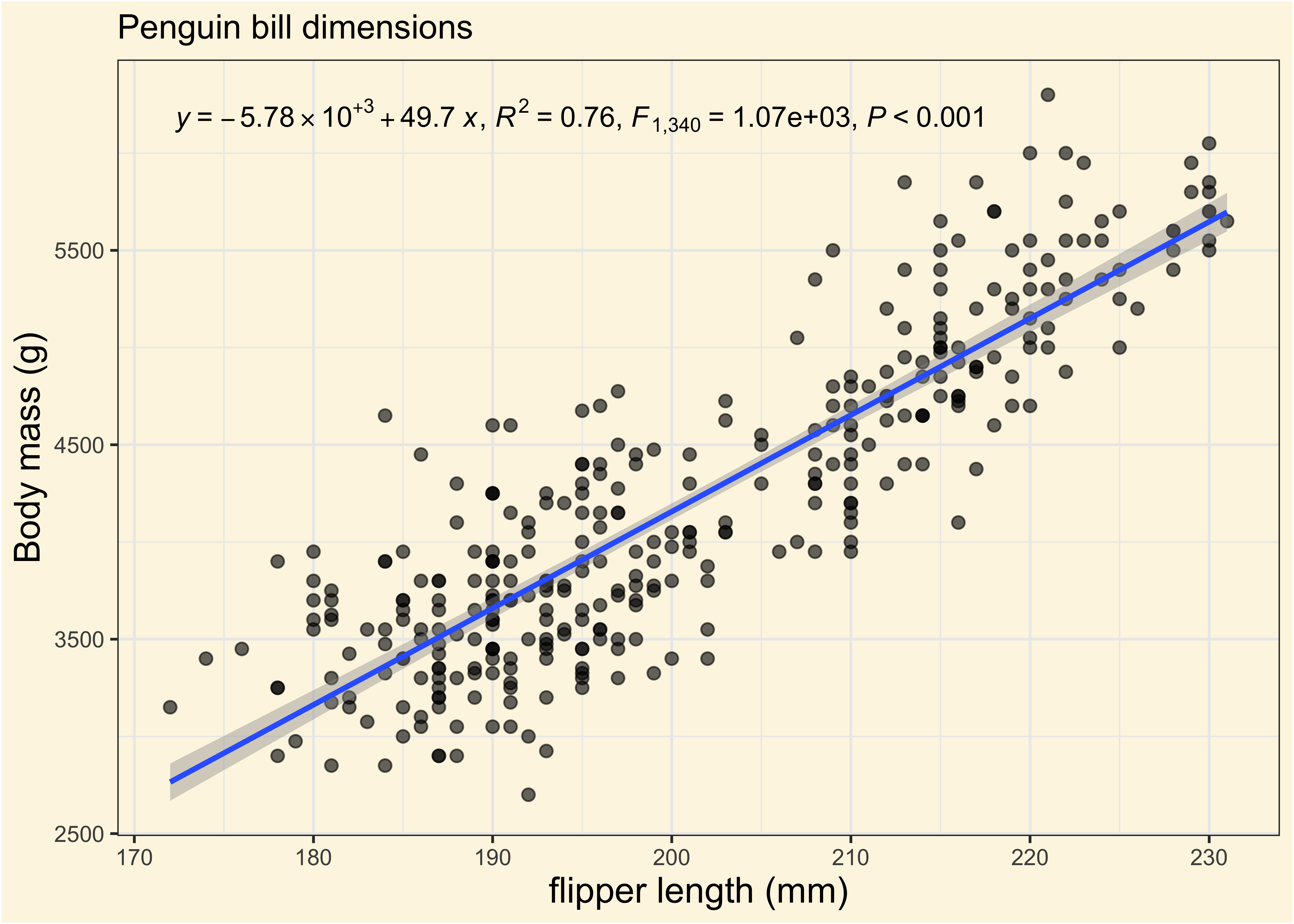
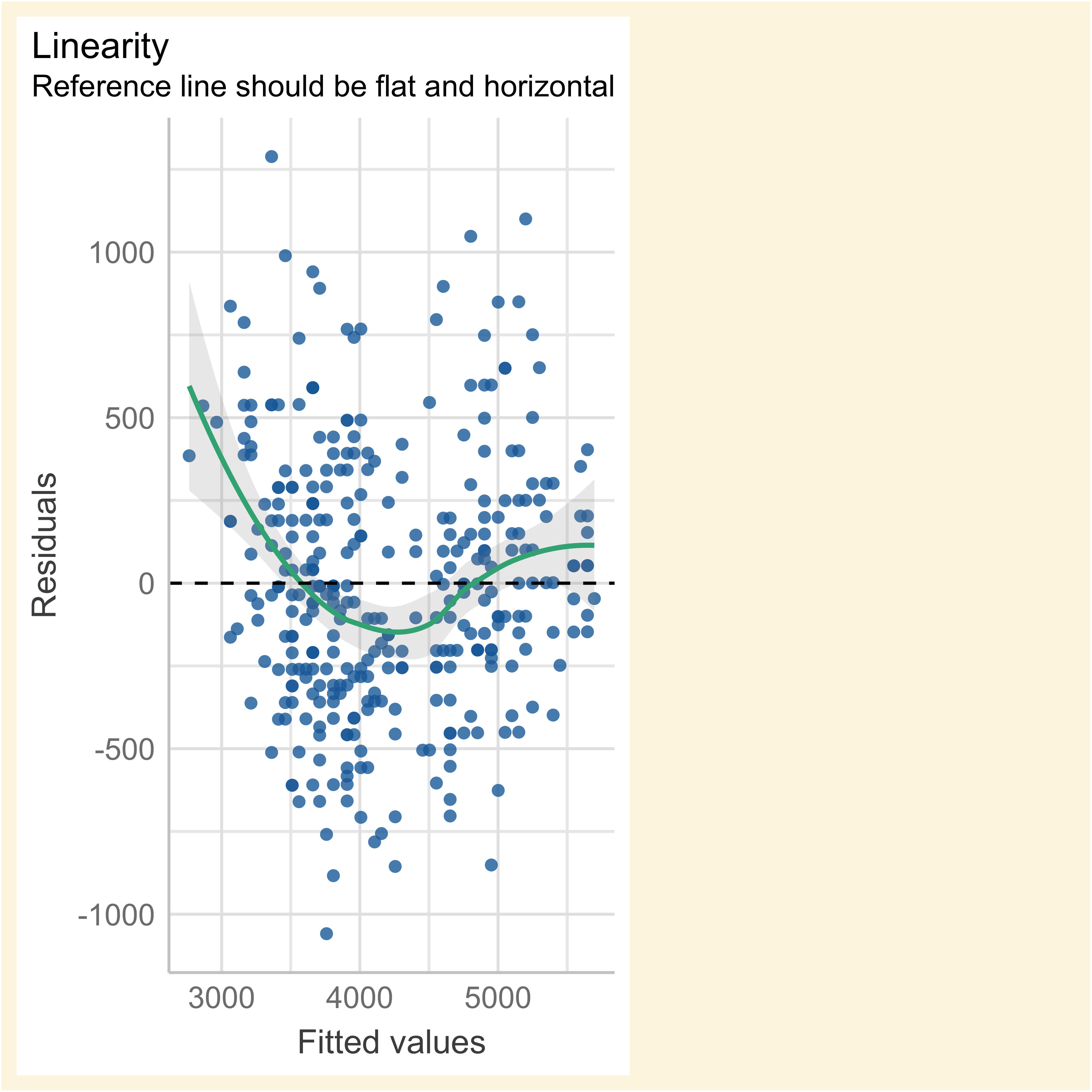
We fitted a linear model (estimated using OLS) to predict body_mass_g with
flipper_length_mm (formula: body_mass_g ~ flipper_length_mm). The model
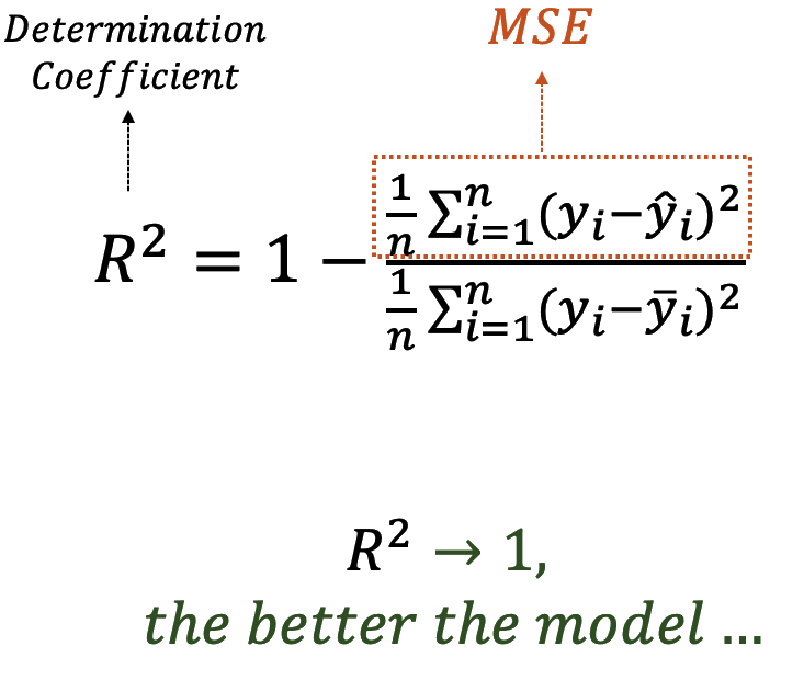
explains a statistically significant and substantial proportion of variance (R2
= 0.76, F(1, 340) = 1070.74, p < .001, adj. R2 = 0.76). The model's intercept,
corresponding to flipper_length_mm = 0, is at -5780.83 (95% CI [-6382.36,
-5179.30], t(340) = -18.90, p < .001). Within this model:

  - The effect of flipper length mm is statistically significant and positive
(beta = 49.69, 95% CI [46.70, 52.67], t(340) = 32.72, p < .001; Std. beta =
0.87, 95% CI [0.82, 0.92])

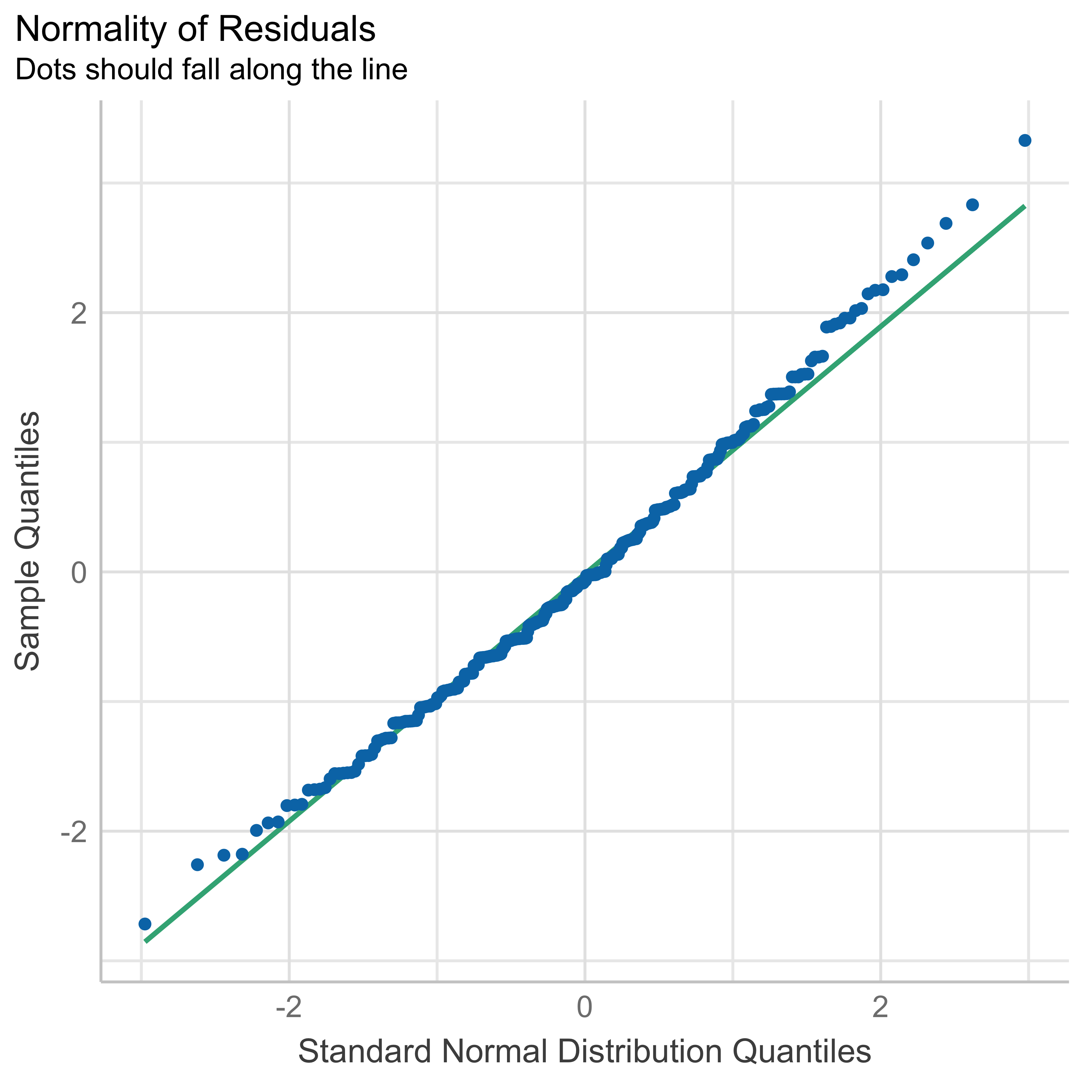
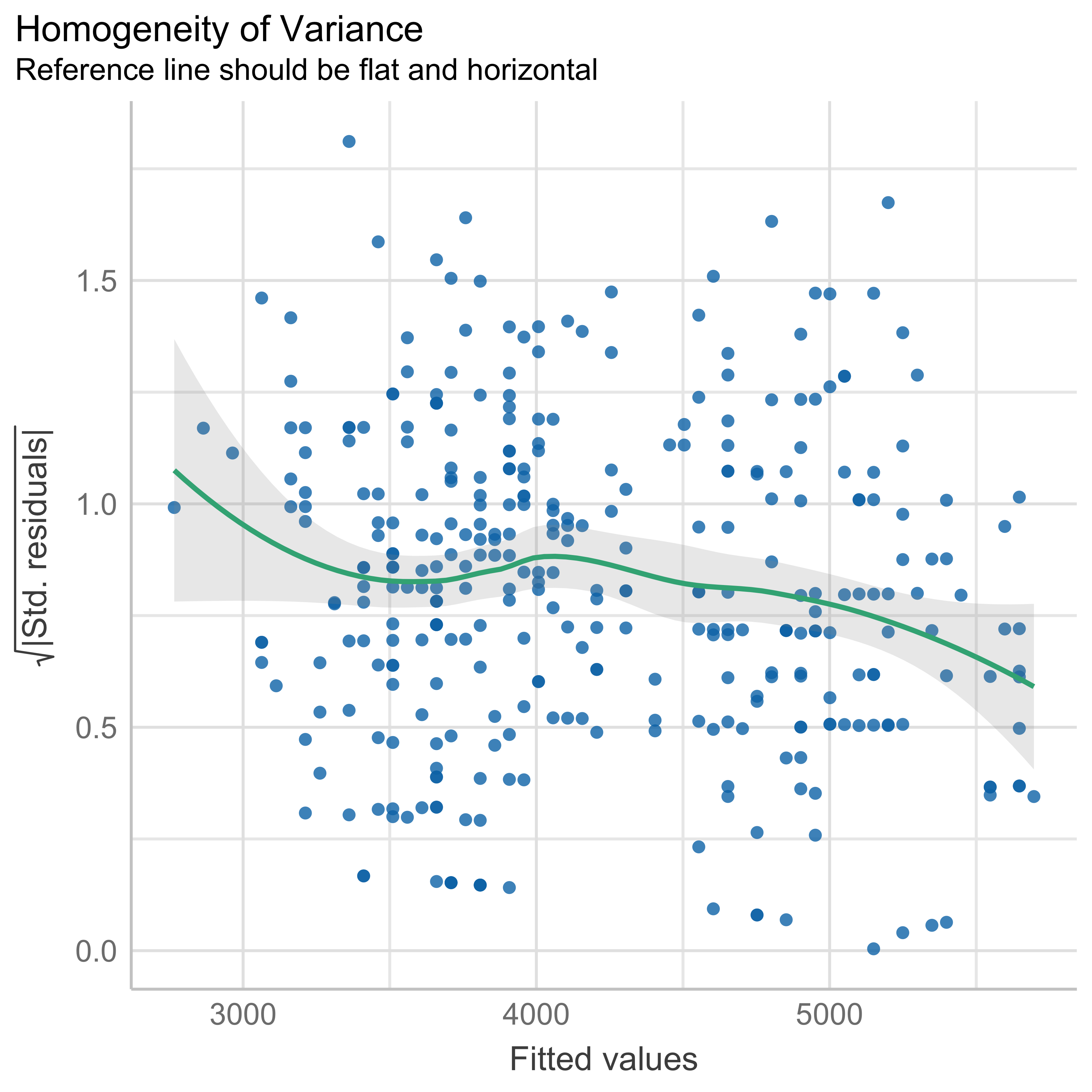
Standardized parameters were obtained by fitting the model on a standardized
version of the dataset. 95% Confidence Intervals (CIs) and p-values were
computed using a Wald t-distribution approximation.

We can also include the complete model in the plot with the ggpmisc:

ggplot(penguins, 
  aes(
      x = flipper_length_mm, 
      y = body_mass_g)
      ) +
    geom_point(size = 2, alpha = 0.6) +
    labs(
        title = "Penguin bill dimensions",
        x = "flipper length (mm)",
        y = "Body mass (g)"
    ) +
    geom_smooth(method = "lm") +
    stat_poly_eq(use_label(
      c("eq", "R2", "F", "p.value"),
    ))

Testing the regression assumtions

1. Linearity: function behaves linearly outside the range of the data.

performance::check_model(model, check = "linearity")

2. Normality: residuals are normally distributed.

performance::check_normality(model)

OK: residuals appear as normally distributed (p = 0.109).

plot(check_normality(model), type = "qq")

3. Variance homogeneity: residuals have constant variance.

check_heteroskedasticity(model)

OK: Error variance appears to be homoscedastic (p = 0.140).

plot(check_heteroskedasticity(model))