GLM & AIC

https://tinyurl.com/29wkzwwj

Camilo G.

ca.garcia2@uniandes.edu.co

Alejandra S.

m.soto2@uniandes.edu.co

Ronald D.

r.diazf@uniandes.edu.co

Andrew C.

aj.crawford244@uniandes.edu.co

Mauricio S.

om.santos@uniandes.edu.co

Generalized Linear Models (GLM)

We have assume data (and residuals) follow a normal distribution for regular lineal models, but what if that does not always happen?

1. Structural component (\(\eta = \beta x\))

2. Link function (\(\eta = g(\mu)\))¹

3. Random component (Normal, Binomial, Poisson, Neg. Binomial, etc.)

1. An equation that delinearizes the mathematical relationship between the predictor and the outcome. It is a transformation of the predictors

What regression should we apply?

It depends on the outcome datatype and on the errors distribution of the model.

Regression	Outcome variable	Errors distribution	Link function
Regular/Estandar	Continuos	Normal	Indentity
Logistic	Discrete (two-level factor - binary)	Binomial	Logit
Poisson	Skewed discrete (counts)	Poisson	Log
Neg. Binomial	Discrete (counts)	Neg. Binomial	Inverse
Gamma	Skewed positive continuous	Gamma	Reciprocal

Let’s try it in R:

adelies <- penguins |>
  filter(species == "Adelie") |>
  drop_na() |>
  mutate(binarysex = case_when(
    sex == "male" ~ 1,
    sex == "female" ~ 0
  ))

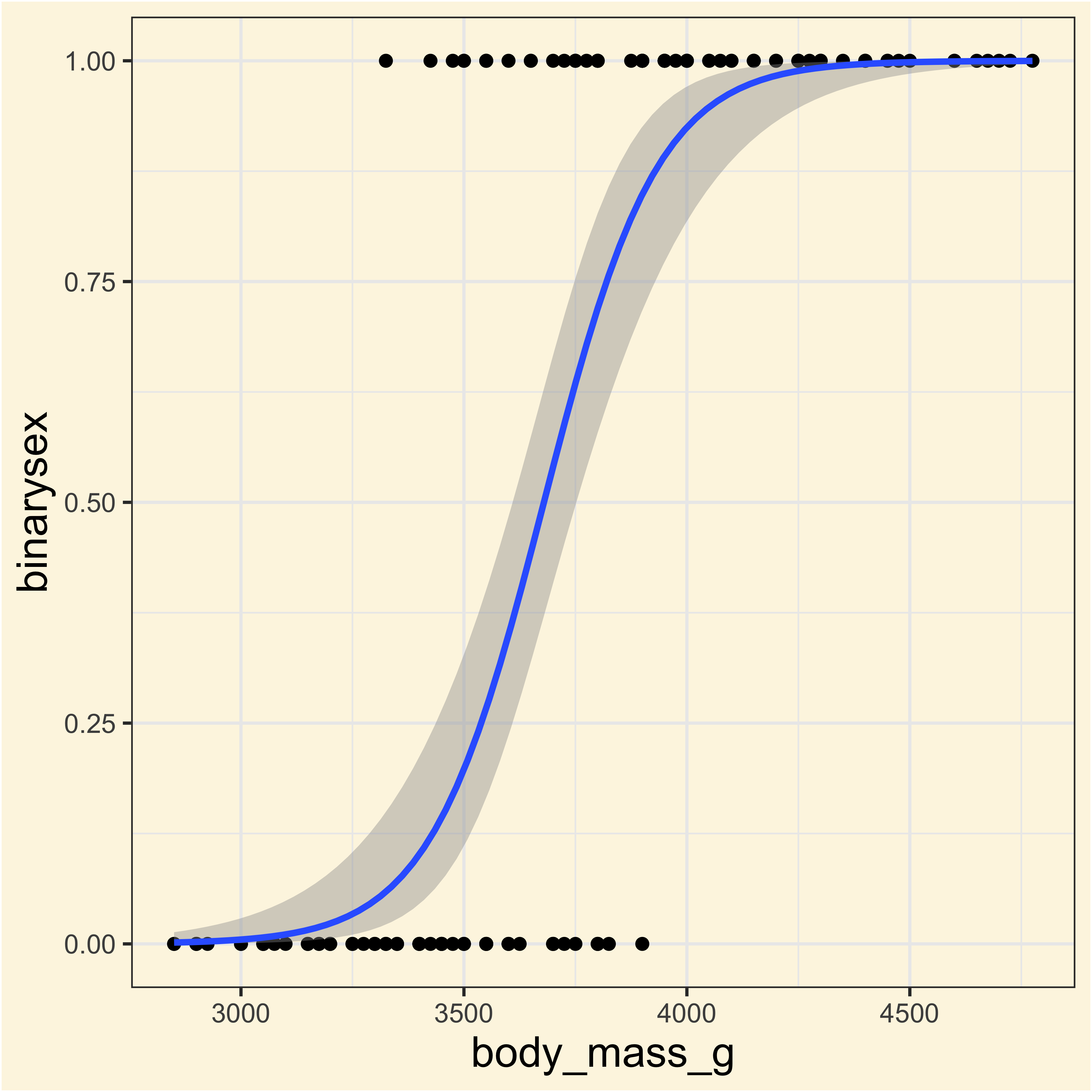
Let’s create the GLM for to predict a penguin’s sex based on it’s body mass:

binarysexmodel <- glm(binarysex ~ body_mass_g, data = adelies, family = "binomial")

Let’s see what the outout is:

Call:  glm(formula = binarysex ~ body_mass_g, family = "binomial", data = adelies)

Coefficients:
(Intercept)  body_mass_g  
 -28.749639     0.007814  

Degrees of Freedom: 145 Total (i.e. Null);  144 Residual
Null Deviance:      202.4 
Residual Deviance: 88.74    AIC: 92.74

What did we do?

report::report(binarysexmodel)

We fitted a logistic model (estimated using ML) to predict binarysex with
body_mass_g (formula: binarysex ~ body_mass_g). The model's explanatory power
is substantial (Tjur's R2 = 0.61). The model's intercept, corresponding to
body_mass_g = 0, is at -28.75 (95% CI [-39.49, -20.42], p < .001). Within this
model:

  - The effect of body mass g is statistically significant and positive (beta =
7.81e-03, 95% CI [5.55e-03, 0.01], p < .001; Std. beta = 3.58, 95% CI [2.54,
4.92])

Standardized parameters were obtained by fitting the model on a standardized
version of the dataset. 95% Confidence Intervals (CIs) and p-values were
computed using a Wald z-distribution approximation.

Let’s put that on a plot

ggplot(
  adelies,
  aes(x = body_mass_g, y = binarysex)
) +
  geom_point() +
  geom_smooth(
    method = "glm",
    method.args = list(
      family = "binomial"
    )
  )

Akaike Information Criteria (AIC)

An information theory concept that evaluates mathematical models in terms of its complexity and performance (prediction):

\[AIC=−2*ln(L)+2*k\]

Using Broom to evaluate statistical models.

Tidying model’s statistical information and report their performance.

1. tidy() Summarizes and organize the model information

2. augment() Displays all model information for each data point.

3. glance() Summarizes the model performance (AIC, BIC, and others).

broom::tidy(binarysexmodel)

broom::augment(binarysexmodel)

Now let’s see the AIC:

broom::glance(binarysexmodel)