Seq. Analysis challenges

Seq. Analysis challenges

Counting features

The first step in this journey is to download a bunch of sequences programmatically. To do so, we will use the program ncbi-genome-download.

You could inspect all the options it provides, now we will set our command as the following:

#| echo: true
#| eval: false
ngd --genera "Bacillus subtilis"\
    -s refseq\
    -l complete\
    -o Data\
    --flat-output\
    --format features\
    -n bacteria\
    | head -n 5

To this date this command will search for 216 complete genome information of Bacillus subtilis strains and download the feature-table file compressed. So the next step is to decompress all of them:

for i in *.txt; do
  gzip -d $i
done

Now the the feature-table file is a is a long table containing each of the features annotated in the genome see the top of a file:

head -n 5 data/features/GCF_000009045.1_ASM904v1_feature_table.txt

# feature   class   assembly    assembly_unit   seq_type    chromosome  genomic_accession   start   end strand  product_accession   non-redundant_refseq    related_accession   name    symbol  GeneID  locus_tag   feature_interval_length product_length  attributes
gene    protein_coding  GCF_000009045.1 Primary Assembly    chromosome      NC_000964.3 410 1750    +                   dnaA    939978  BSU_00010   1341        old_locus_tag=BSU00010
CDS with_protein    GCF_000009045.1 Primary Assembly    chromosome      NC_000964.3 410 1750    +   NP_387882.1 WP_003242674.1      chromosomal replication initiator informational ATPase  dnaA    939978  BSU_00010   1341    446 
gene    protein_coding  GCF_000009045.1 Primary Assembly    chromosome      NC_000964.3 1939    3075    +                   dnaN    939970  BSU_00020   1137        old_locus_tag=BSU00020
CDS with_protein    GCF_000009045.1 Primary Assembly    chromosome      NC_000964.3 1939    3075    +   NP_387883.1 WP_003242509.1      DNA polymerase III (beta subunit)   dnaN    939970  BSU_00020   1137    378

The question now is how to count the lines corresponding to features which is the first line. It contains six types of features (CDS, gene, rRNA, tRNA, tmRNA, ncRNA and misc_RNA). This task could be achieved by many ways, but a general approach to count lines is the way through it. Here there three approaches to follow:

#! usr/bin/bash

export features="id CDS gene ncRNA rRNA tmRNA tRNA"

echo $features


for i in $(ls $1); do
    values=$(awk '/CDS/{++cnt1} /gene/{++cnt2} /ncRNA/{++cnt3} /rRNA/{++cnt4} /tmRNA/{++cnt5} /tRNA/{++cnt} END {print cnt1, cnt2, cnt3, cnt4, cnt5, cnt6}' ${1}/${i});
    id=$(egrep -o -m 1 "GCF.{12}" ${1}/${i})
    echo "$id $values"
done

id CDS gene ncRNA rRNA tmRNA tRNA
GCF_000009045.1 4238 4578 4 76 2 
GCF_000146565.1 3998 4120 6 64 2 
GCF_000186745.1 4111 4247 6 78 2 
GCF_000209795.2 4262 4400 6 76 2 
GCF_000227465.1 4167 4314 6 76 2 
GCF_000227485.1 3991 4128 6 76 2 
GCF_000293765.1 4205 4343 6 76 2 
GCF_000321395.1 4043 4179 6 76 2

library(tidyverse)
library(fs)

all_features <- dir_ls("data/features/") |> # GCF_000186745.1_ASM18674v1_feature_table.txt is corrupted
  map_df(read_tsv)

all_features |> 
  head()

Now that we read all the files into the programming environment we can operate over them with different libraries.

all_features_grouped <- all_features |> 
  rename(feature = `# feature`) |>
  select(assembly, feature) |>
  group_by(assembly, feature) |>
  count() |>
  pivot_wider(names_from = feature, values_from = n)

all_features_grouped

1: Change the # feature name for simple feature.
2: Select feature and assembly columns.
3: Group by these two columns, enabling grouping operations.
4: Count the numbers of rows based on the applied grouping.
5: Generate a wide dataset sending row names as columns.

import glob
import pandas as pd

files = glob.glob("data/features/*.txt")

df = pd.concat((pd.read_csv(f, sep='\t') for f in files))

df_renamed  = df.rename(columns={"# feature" : "feature"})

df_filtered = df_renamed.filter(items=["feature", "assembly"])

df_filtered.groupby(["assembly","feature"])["feature"].count()

Sanger processing

Processing a Sanger AB1 file is a very common task in bioinformatics, yet it is sometimes taked for grandted. Many graphical programs allow to process the sequences, yet the task are currently manual involving the trimming and reverse complement generation of the reverse reads (when pair-end sequencing). But, given the vast generation of data on the present, Sanger sequencing is used massively in parallel to generate huge amount of sequences. Therefore, processing “by-hand” becomes an unachivable task.

Several programs have been developed to automate the processing of sequences, an open source library in R is sangeranalyseR.

library(sangeranalyseR)

Processing a single gene `AB1` pair

rpoB <- SangerAlignment(
  ABIF_Directory = "data/sanger-seqs/rpoB/",
  REGEX_SuffixForward = "rpoB_1_F.ab1",
  REGEX_SuffixReverse = "rpoB_2_R.ab1",
  TrimmingMethod = "M2",
  M2CutoffQualityScore = 33,
  M2SlidingWindowSize = 5
)

rpoB

SangerAlignment S4 instance
           Input Source :  ABIF 
         Process Method :  REGEX 
         ABIF Directory :  data/sanger-seqs/rpoB/ 
   REGEX Suffix Forward :  rpoB_1_F.ab1 
   REGEX Suffix Reverse :  rpoB_2_R.ab1 
      Contigs Consensus :  TTTTTTTTTTTTTTTTTTTTTTTTTTTTTTKGGGGGGGAGWACTTGAGGAGCCATCATCATGAGTGAACGTCTTGTGAAGGATGATGTTTATACATCTATCCATATTGAAGAATATGAATCAGAAGCACGTGATACGAAACTTGGACCTGAAGAAATCACTCGCGATATTCCAAACGTCGGTGAAGATGCGCTTCGCAATCTTGATGACCGCGGAATCATCCGTATTGGGGCAGAAGTAAAAGACGGAGATCTTCTTGTTGGTAAAGTAACGCCTAAAGGTGTAACCGAACTGACTGCTGAAGAACGCCTTCTTCACGCCATCTTTGGTGAAAAAGCCCGCGAGGTTCGTGATACTTCTCTTCGTGTGCCTCACGGCGGCGGCGGAATTATCCACGACGTTAAAGTCTTCAACCGTGAAGACGGAGACGAACTTCCTCCAGGTGTAAACCAGTTGGTACGCGTATATATCGTTCAGAAACGTAAGATTTCTGAAGGGGATAAAATGGCCGGTCGTCACGGTAACAAAGGTGTTATCTCTAAGATTCTTCCTGAAGAGGATATGCCTTACCTTCCTGACGGCACACCAATTGACATCATGCTTAACCCGCTGGGCGTACCATCACGTATGAACATCGGGCAGGTATTGGAGCTTCATATGGGTATGGCCGCTCGTTACCTCGGCATTCACATTGCGTCTCCTGTATTTGATGGAGCGCGAGAAGAGGATGTTTGGGAAACACTTGAAGAAGCCGGCATGTCTCGTGACGCCAAAACGGTGCTTTACGACGGACGTACTGGAGAGCCGTTTGATAACCGCGTGTCTGTCGGTATCATGTACATGATCAAACTGGCACACATGGTTGACGATAAACTTCATGCACGCTCTACAGGTCCTTACTCACTTGTTACGCAGCAGCCTCTTGGCGGTAAAGCGCAATTTGGCGGACAGCGTTTTGGTGAGATGGAGGTTTGGGCACTTGAAGCTTATGGTGCAGCTTACACTCTTCAAGAAATTCTGACTGTTAAGTCCGATAACGTGGTTGGACGTGTGAAACTACACCTCDSTGGCACAAAAAAAAAAAAAAAAAAAAAAAAAAAAAAA

This produces an specialized R object holding different information from the Sanger processing steps. The entire object can be untangled in a thorough report displaying all the processing information and results using the

generateReport(rpoB, outputDir = "data/sanger-processed/")

Among the data from the report ypu can see that the unaligned contigs ithere is something called a Contig Consensus which is the result of comparing the three consensus out of the rpoB genes of the three strains (302, 321, 455). Now, this is not really the sequence we need right away, however we need the separate consensus of each strain gene. To get theme sangeranalyseR provide a couple of tools.

writeFasta(rpoB,
  outputDir = "data/sanger-processed/rpoB",
  selection = "contigs_unalignment",
)

Now, in the case of the challenge we actually got several genes per strain which is common in molecular biology projects. How do we process all the batch of sequence all at a time? To do so we can split the sequences as folder per gene, then we can use some capabilites of are to iterate an map the sanger processing function to each folder and create a list of processing instances, let’s try this out:

Processing a bulk of `AB1` pair

library(fs)
library(purrr)

dirs <- fs::dir_ls("data/sanger-seqs/")


sanger_bulk <- function(dir) {
  SangerAlignment(
    ABIF_Directory = dir,
    REGEX_SuffixForward = "_1_F.ab1",
    REGEX_SuffixReverse = "_2_R.ab1",
    M2CutoffQualityScore = 33,
    M2SlidingWindowSize = 2
  )
}

genes <- dirs |> 
  map(sanger_bulk)

genes$

genes$`data/sanger-seqs/rpoB`

NULL

genes$`data/sanger-seqs/spo0B`

SangerAlignment S4 instance
           Input Source :  ABIF 
         Process Method :  REGEX 
         ABIF Directory :  data/sanger-seqs/spo0B 
   REGEX Suffix Forward :  _1_F.ab1 
   REGEX Suffix Reverse :  _2_R.ab1 
      Contigs Consensus :  ATCAACCATGCCAGAAAAAAGGAACATGATATTTCTGGGAAAAACMATTGTTTTTCTAACAAAGCCTTACTCTGTTATAATTCATAATACACACTTATACAGACTCCTAAATAAGAAATTAAATGATTGGGAGTGCGAAAATGAAGGATGTTTCAAAAAATCAAGAAGAAAATATAAGCGACACGGCATTAACAAACGAACTGGTTCATCTGCTGGGCCATTCCCGGCATGATTGGATGAATAAGCTGCAGCTGATTAAAGGAAACTTAAGCTTGCAGAAGTATGACCGCGTCTTTGAAATGATTGAAGAAATGGTTATAGACGCGAAGCACGAATCAAAGCTCTCAAACCTAAAAACACCGCATTTGGCGTTTGATTTTCTTACATTTAATTGGAAAACCCATTATATGACGCTTGAATATGAAGTTCTTGGAGAAATTAAGGATTTGTCGGCTTATGATCAAAAGCTGGCAAAACTGATGAGAAAGCTGTTTCATCTGTTTGATCAAGCAGTCAGCAGAGAGAGTGAAAATCATTTAACGGTTTCGCTTCAAACAGATCATCCTGACAGACAGCTGATTCTGTACCTTGATTTTCACGGCGCCTTTGCCGATCCTTCTGCTTTTGATGATATTCGGCAGAATGGATACGAGGATGTGGATATCATGCGTTTTGAGATCACAAGCCACGAATGTCTGATTGTAAATAGGGTTGGTACTAGCGGTAGTTTTTAACGGTTTAGAACGGAGGACATTATGTTTGTAGATCAGGTCAAAGTATATGTAAAAGGCGGCG

Finally to generate reports we need to call the appropriate instance with the $ to select the gene we are interested to inspect:

generateReport(genes$`data/sanger-seqs/spo0B`, outputDir ="data/sanger-processed/spo0B")


writeFasta(
 genes$`data/sanger-seqs/rpoB`,
 outputDir = "data/sanger-processed/rpoB",
 selection = "contigs_unalignment"
)

Now that we got the actual multifasta of the genes from all strain, the identification process using blastn from the command line will follow as:

blastn -db nr -query rpoB-unaligned-contigs.mfa -out rpoB-blastn-report.txt -remote

Multiple sequence alignment

Download sequences

Make sure to use the --flat-output avoiding download of multiple metadata

ngd --flat-output -p 4 -s refseq -A genome-accessions.txt -F cds-fasta bacteria

In this case cds-fasta parameter will download the nucleotide sequences of the gene. Other alternatives could be useful such as blast search on a genome database or searching through the GENBANK annotation files (both files also could be downloaded using ngd).

Unwrapping FASTA records

NCBI registries came with an undesirable wrapping around the lines of sequencing which basically is inserting a return character after some established number of characters. Then a way to get rid of them is to use a command line utility from AstrobioMike (Mike Lee) which will give a line per sequence after the FASTA header. We can later assume the the first line after the header will be the entire sequence

for i in GCF_*; do 
    N=$(basename $i .fna); 
    bash bit-remove-wraps.sh ${i} > ${N}_unwrapped.fasta; 
done

Gene searching

A possible way to search throughout the file registries is by using the grep command, that recursively will search each file. Fine tuned it allow to search for the first match, but also for the “after-context” in terms of lines desired to be printed:

for i in *unwrapped*; do grep -A 1 "gyrA" $i; done > all-gyrA.fasta

After finding the genes, we are now with an almost clean multi-sequence file, because header names are still and will be problematic. How do we programmatically change the FASTA headers? We will see in the next step.

Now the the files has files names that are simply to work with. Which will enable to asses better out sequence alignment matrix.

Sequence alignment

There are many programs that are suited for performed multiple sequence alignments. Perhaps the two most used are MAFFT and MUSCLE both specialized in multiple sequence alignment (that is: when having two or more than two sequences). The second tends to be more accurate when having large data-sets, but the first on is more versatile, fast and accurate on different kind of data-sets.

Both programs take as input a single file containing all the sequences concatenated horizontally (that is a multi-fasta file) careless of the extension but (MFA, FA, FASTA, FNA, etc). And generate a simple output (whether with the -o in MUSCLE or to the std output in MAFFT)

linsi --preservecase --reorder all-gyrA-renamed.fasta > all-gyrA-renamed-linsi.fasta # locally

Tip

Other alignment alternatives are:

muscle -i all-gyrA-renamed.fasta -o all-gyrA-renamed-muscle.fasta

famsa -t 8 all-gyrA-renamed.fasta > all-gyrA-renamed-famsa.fasta

kalign -i all-gyrA-renamed.fasta -o all-gyrA-renamed-kalign.fasta

Assessment of the alignment

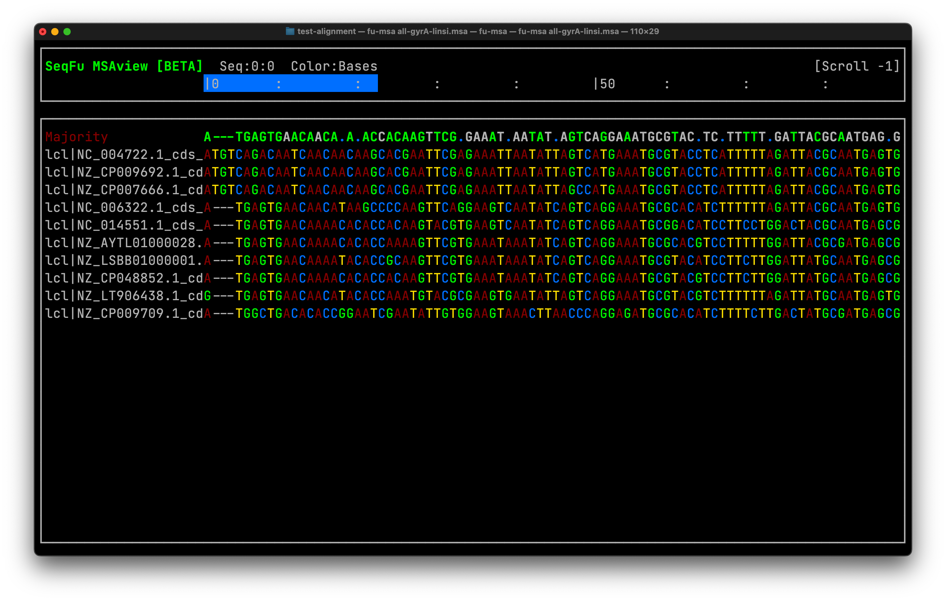
Inspection of the alignment is there very first step for assessing its quality. A CDS tends to generate a codon-like alignment starting with the methionine codon (ATG,GTG) and finishing with a stop (TAA, TAG, etc.). Therefore finding this structure when aligning a complete genes is expected. If a middle fraction of the gene is being aligned ORF might not display any stop codon. Verifying a codon-like alignment shows a biological order on the sequences other that mere artifact of the alignment, that is an evolutionary behavior of the sequence. We can do it using seqfu from the CLI Fig. 1, or interactively with AliView

Figure 1: A viusalization of the *gyrA* gene alignment using seqfu multiple sequence alignment viewer

A second step is to find the variability of the alignment. A simple way to find that is to calculate simpl stats from the alignment (sites, variable sites, As, Ts, etc.). A powerful cli program to do so is goalign

goalign stats -i all-gyrA-renamed-linsi.fasta

length  2508
nseqs   8
avgalleles  1.7400
variable sites  1202
char    nb  freq
-   273 0.013606
A   6418    0.319876
C   3633    0.181071
G   4755    0.236992
T   4985    0.248455
alphabet    nucleotide

Tip

A more in depth analysis of the alignment could be done with CIAlign.