9 Sanger analysis
This is a section about perhaps one of the first generation sequencing technology, that is Sanger sequencing and its principles and evolution, strengths and limitations
This chapter will also cover the bioinformatics side of the method: what kind of files we get out Sanger, how we process them and an important paradigm that came out from this sequence method.
Finally we will dive into a study case that its very common in microbiology: the use of the 16S rRNA gene for taxonomy identification
9.1 The first sequencing methods
Back in 70s there two different methods aiming to determine the base sequences of DNA and they basically operated at the level of base per base reconstruction of the information. The most used during those days was so called :Maxam-Gilbert method and the second one was precisely the chain termination method or dideoxy sequencing or more commonly nowadays :Sanger sequencing. Both methods named after their creators. It was, however the Sanger method the one that gradually became the facto method and continue to be the standard for the next thirty years. In fact, assembled genomes before the 2000s were sequenced with Sanger method, which included the first draft of the Human genome and many other organism Brown (2018).
9.1.1 The chain termination method
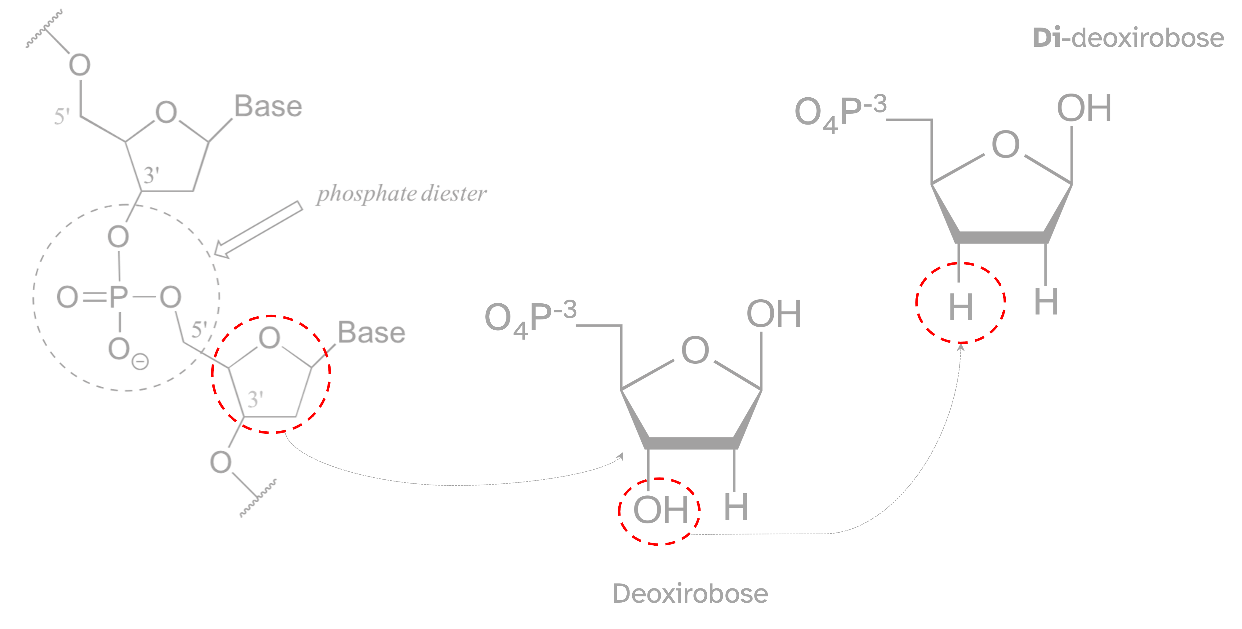
To under stand the chain termination method is important have a clear view of the DNA structure and chemical reaction that enable its polymerization. Whe the
9.1.2 Sanger with capillary electrophoresis
9.1.3 Strengths and limitations of Sanger methods
9.2 Files from Sanger sequencing
Several files are generated from a modern Sanger sequencing project.
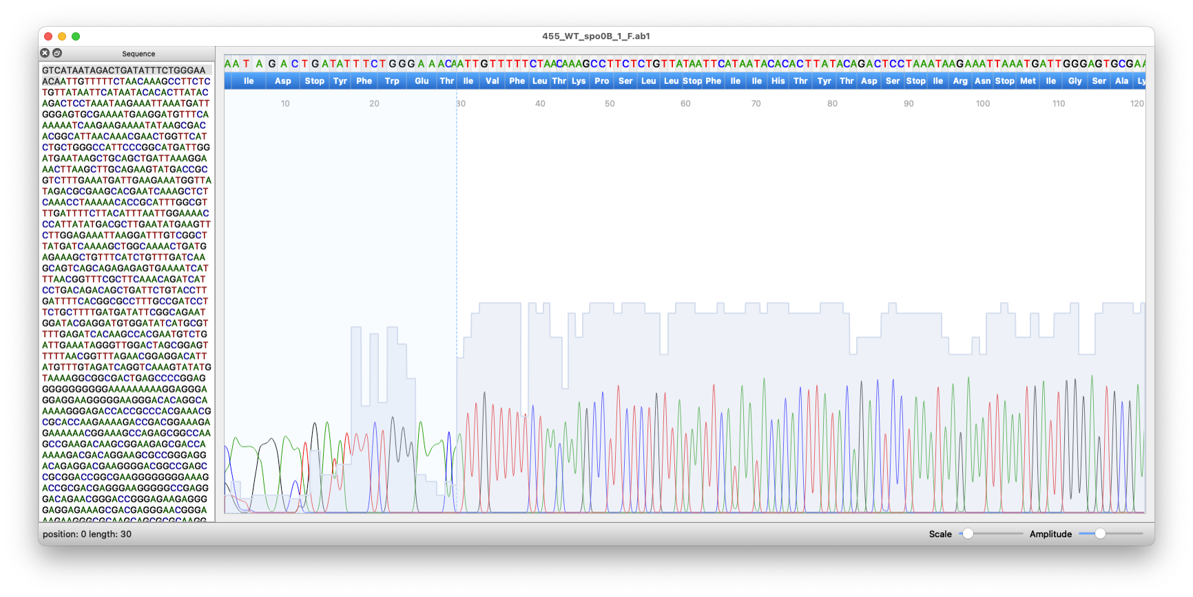
However the most used file is the binary version AB1 which could be red out from different programs including cutepeaks. It displays the DNA sequence along with its quality peak in each position Fig. 9.4
9.3 Sanger processing workflow
Despite being one of the oldest sequencing methods, Sanger sequencing has some remarkable strengths that are enable thanks to the automation era. For instance modern sequencers working in parallel can read almost 384 different sequences (of 750bp) in 1h (7Mb in 24h per machine), clearly automation introduces a second advantage and that is the low-price of sequencing small fragments Brown (2018). It is important to highlight some limitations as well like the necessity of round-the-clock technical support (this also leverages a little bit from robotic operators though). The error-free Sanger sequencing requires at least 5X of sample coverage, which could be seen as disadvantage too Brown (2018).
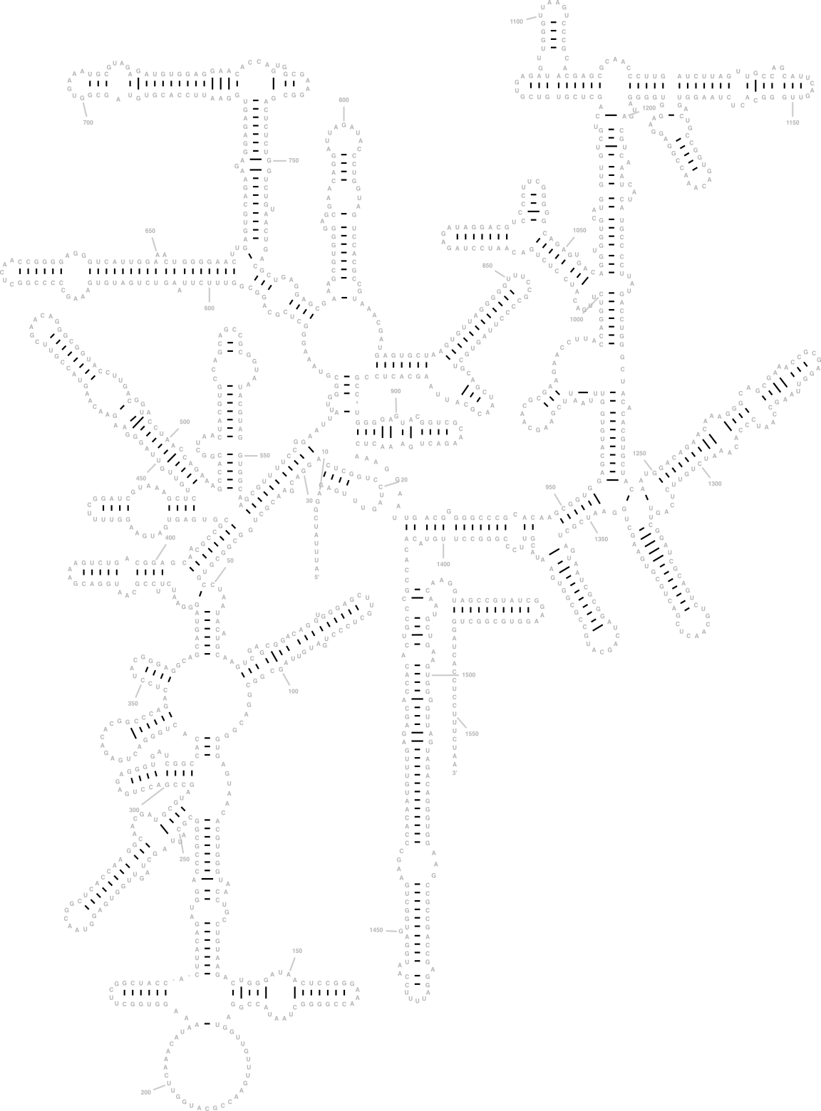
9.4 The 16S rRNA and its relevance for sequencing
Professor Valeska gives you a compressed file containing two genes (spo0B and rpoB) from three different strains (302, 321, 455). These genes were sequenced using pair end Sanger method, then the compressed file has the two raw sequences per gene. She tells you to process and analyse them using the Sanger sequencing pipeline analyis. Since she doesn’t know from which species they belong, she ask you to identify the organism to whom it belongs by using the resulting consensus sequence. She finally reminds you to document each step of the process including the identification step
See the solution :here


